$$ \newcommand{\AbsoluteConicImageEntry}{B} \newcommand{\AbsoluteConicImageMatrix}{\mathbf{B}} \newcommand{\AbsoluteConicVector}{\mathbf{b}} \newcommand{\AcceleratedEpisodeTime}{T'} \newcommand{\AcceleratedFractionSpeedup}{G} \newcommand{\AccelerationNoiseDensityMatrix}{\mathbf{Q}_c} \newcommand{\AccelerationNoiseSpectralDensity}{q_c} \newcommand{\AccelerationWhiteNoise}{w} \newcommand{\AcceleratorBatchTime}{T_{\text{GPU}}} \newcommand{\AcceleratorConsumptionRate}{R_{\text{accel}}} \newcommand{\AcceleratorCount}{N_{\text{GPU}}} \newcommand{\AcceleratorDataConsumptionRate}{R_{\text{consumption}}} \newcommand{\AcceleratorGain}{G_{\text{accel}}} \newcommand{\AcceleratorHourlyPrice}{R_{\text{GPU/hr}}} \newcommand{\AcceleratorMemoryBandwidth}{\text{BW}_{\text{accelerator}}} \newcommand{\AcceleratorRailVoltage}{V_{\text{rail}}} \newcommand{\AcceleratorSecondsPerQuery}{S_{\text{GPU/query}}} \newcommand{\AcceleratorSupplyCurrent}{i} \newcommand{\AcceleratorTargetQueryRate}{R_{\text{GPU,target}}} \newcommand{\AcceleratorsPerNode}{G_{\text{node}}} \newcommand{\AccelerometerBias}{b_a} \newcommand{\AcceptanceFraction}{\alpha} \newcommand{\AcceptanceIntervalLowerLimit}{L} \newcommand{\AcceptanceIntervalUpperLimit}{U} \newcommand{\AcceptanceProbability}{p_{\text{acc}}} \newcommand{\AcceptedInfluences}{\text{Inf}} \newcommand{\AcceptedInputSet}{\mathcal{A}_{\tau}} \newcommand{\AcceptedLabelCount}{d} \newcommand{\AcceptedOutcomePayoff}{V} \newcommand{\AcceptedSampleCount}{X} \newcommand{\AcceptedTaskMeanCost}{C_{\text{succ}}} \newcommand{\AcceptedTasks}{N_{\text{acc}}} \newcommand{\AcceptingStateSet}{F} \newcommand{\AccessAttemptTime}{t} \newcommand{\AccountQueryDistribution}{p_{\text{user}}} \newcommand{\AccumulatedProcessNoiseCovariance}{\mathbf{Q}_d} \newcommand{\AccumulatedSyncTime}{T_{\text{sync}}} \newcommand{\AccumulatedUpdateTime}{T_{\text{effective}}} \newcommand{\AccumulationStepCount}{k} \newcommand{\AccuracyAfterDeployment}{\text{Accuracy}} \newcommand{\AccuracyDecayRate}{\gamma} \newcommand{\AccuracyPayoffPerQuery}{V} \newcommand{\AchievedBrakingDeceleration}{a} \newcommand{\AchievedKernelBandwidth}{\text{BW}_{\text{effective}}} \newcommand{\AcquisitionEpoch}{t_{\text{acq}}} \newcommand{\ActVariationalObjective}{\mathcal{L}_{\text{ACT}}} \newcommand{\ActionBinCount}{B} \newcommand{\ActionChunk}{\mathbf{A}} \newcommand{\ActionChunkHorizon}{H} \newcommand{\ActionChunkIndex}{k} \newcommand{\ActionDimension}{d_a} \newcommand{\ActionExecutionRate}{f_{\text{exec}}} \newcommand{\ActionFilterCutoffFrequency}{f_{\text{cutoff}}} \newcommand{\ActionLowerBound}{\mathbf{a}_{\min}} \newcommand{\ActionMagnitudeBound}{a_{\max}} \newcommand{\ActionRangeMaximum}{a_{\max}} \newcommand{\ActionRangeMinimum}{a_{\min}} \newcommand{\ActionRecoverableFraction}{\rho_{a}} \newcommand{\ActionResidualVector}{\mathbf{r}} \newcommand{\ActionSpace}{\mathcal{A}} \newcommand{\ActionTokenPrefix}{a_{<j}} \newcommand{\ActionUpperBound}{\mathbf{a}_{\max}} \newcommand{\ActivationCheckpointCount}{n_{\text{ckpt}}} \newcommand{\ActivationFunction}{f} \newcommand{\ActivationInput}{x} \newcommand{\ActivationLipschitzBound}{L_{\phi}} \newcommand{\ActivationMatrix}{\mathbf{A}} \newcommand{\ActivationMemory}{M_{\text{activations}}} \newcommand{\ActivationPayloadSize}{M_{\text{act}}} \newcommand{\ActivationStagingTime}{t_{\text{activate}}} \newcommand{\ActivationVector}{\mathbf{a}} \newcommand{\ActiveContactIndex}{k} \newcommand{\ActiveControlTorque}{\mathbf{u}_{\text{active}}} \newcommand{\ActiveInferencePower}{P_{\text{active}}} \newcommand{\ActiveLeaseCount}{N_{\text{active}}} \newcommand{\ActiveMotionDuration}{T_{\text{motion}}} \newcommand{\ActiveParameterCount}{P_{\text{model}}} \newcommand{\ActivePrefillRequestSet}{\mathcal{P}_{\text{active}}} \newcommand{\ActiveSchemaSet}{\mathcal{S}} \newcommand{\ActiveTargetTokenCount}{N_{\text{active}}} \newcommand{\ActorAccelerationBound}{a_{k,\max}} \newcommand{\ActorBodyRadius}{r} \newcommand{\ActorUpdateDelayCount}{d} \newcommand{\ActuatedJointAccelerations}{\ddot{\mathbf{q}}_j} \newcommand{\ActuatedJointBiasForces}{\mathbf{h}_j} \newcommand{\ActuatedJointCoordinates}{\mathbf{q}_j} \newcommand{\ActuationSelectionBaseBlock}{\mathbf{S}_b} \newcommand{\ActuationSelectionMatrix}{\mathbf{S}} \newcommand{\ActuatorAxisCount}{N_{\text{axes}}} \newcommand{\ActuatorBiasEffort}{u_{\text{bias}}} \newcommand{\ActuatorCyclePeriod}{t_{\text{cycle}}} \newcommand{\ActuatorDutyCycle}{D_{\text{cycle}}} \newcommand{\ActuatorEffort}{u} \newcommand{\ActuatorOffTime}{t_{\text{off}}} \newcommand{\ActuatorOnTime}{t_{\text{on}}} \newcommand{\ActuatorResponseTime}{T_{\text{act}}} \newcommand{\ActuatorTorqueLowerBound}{\mathbf{u}_{\min}} \newcommand{\ActuatorTorqueUpperBound}{\mathbf{u}_{\max}} \newcommand{\AdamFirstMoment}{m} \newcommand{\AdamMomentDecayRate}{\beta} \newcommand{\AdamSecondMoment}{v} \newcommand{\AdaptationEnergyAllowance}{E_{\text{slack}}} \newcommand{\AdaptationInvestmentCost}{C_{\text{invest}}} \newcommand{\AdaptationLatencyIncrease}{\Delta L_{\text{lat,fg}}^{\text{wc}}} \newcommand{\AdaptationModule}{g_{\psi}} \newcommand{\AdaptationPeakMemory}{M_{\text{peak}}} \newcommand{\AdaptationPowerIncrement}{P_{\text{update}}} \newcommand{\AdaptationWindowEnergy}{E_{\text{update}}} \newcommand{\AdaptedHiddenActivation}{\mathbf{h}'} \newcommand{\AdaptedTaskCost}{C_{\text{task, adapt}}} \newcommand{\AdaptedWeightMatrix}{\mathbf{W}_{\text{adapted}}} \newcommand{\AdapterActivationFunction}{\sigma} \newcommand{\AdapterAssignmentVector}{\mathbf{m}} \newcommand{\AdapterDownProjectionMatrix}{\mathbf{A}} \newcommand{\AdapterIndex}{k} \newcommand{\AdapterInitializationStandardDeviation}{\sigma} \newcommand{\AdapterRank}{r} \newcommand{\AdapterScalingFactor}{\gamma} \newcommand{\AdapterUpProjectionMatrix}{\mathbf{B}} \newcommand{\AdjacentNeighboringDataset}{X'} \newcommand{\AdjacentQueryResult}{v'} \newcommand{\AdminLeaseTime}{T_{\text{admin}}} \newcommand{\AdmissibleBacklogCount}{n} \newcommand{\AdmissibleControlSet}{\mathcal{U}_{\text{adm}}} \newcommand{\AdmissibleDisturbanceSet}{\mathcal{W}} \newcommand{\AdmissionCheckCount}{n_{\text{chk}}} \newcommand{\AdmissionCheckIndex}{i} \newcommand{\AdmissionDecisionEvent}{e_{\text{auth}}} \newcommand{\AdmissionInclusivePrebrakeDelay}{T_{\text{true}}} \newcommand{\AdmissionRouteYield}{Y} \newcommand{\AdmittedAttemptCap}{N} \newcommand{\AdmittedCommand}{u} \newcommand{\AdmittedContactForce}{F^*} \newcommand{\AdmittedControlCommand}{\mathbf{u}} \newcommand{\AdmittedSpeedCommand}{v^*} \newcommand{\AdmittedTargetPosition}{\hat{\mathbf{p}}_{\text{target}}} \newcommand{\AdmittedWorkUnitCount}{m} \newcommand{\AdvantageStabilizer}{\epsilon_{\text{stab}}} \newcommand{\AdversarialDisturbance}{\mathbf{d}} \newcommand{\AdversarialExample}{x_{\text{adv}}} \newcommand{\AdversarialInputLength}{n} \newcommand{\AdversarialPenaltyWeight}{\lambda_{\text{adv}}} \newcommand{\AdversarialPerturbation}{\boldsymbol{\delta}_{\text{adv}}} \newcommand{\AdversarialPerturbationBudget}{\epsilon_{\text{adv}}} \newcommand{\AdversaryLoss}{\mathcal{L}_{\text{adv}}} \newcommand{\AffordanceFrame}{\mathcal{F}_{\text{affordance}}} \newcommand{\AffordanceSuccessEstimate}{V_{\text{policy}}} \newcommand{\AgeBlindTravel}{\Delta x_{\text{blind}}} \newcommand{\AgeCheckInstant}{t_{\text{curr}}} \newcommand{\AggregateServerPower}{P_{\text{servers}}} \newcommand{\AggregateSlotWork}{W} \newcommand{\AggregatedRecoveryDataset}{\mathcal{D}} \newcommand{\AggregatedSurrogateLoss}{\epsilon_N} \newcommand{\AggregationLearnedPolicy}{\hat{\pi}} \newcommand{\AggregationLearnerStateDistribution}{d_{\hat{\pi}_i}} \newcommand{\AggregationRoundCount}{N} \newcommand{\AggregationRoundIndex}{i} \newcommand{\AggregationRoundTrajectorySet}{\mathcal{T}} \newcommand{\AiStandaloneSensitivity}{S_{\text{AI}}} \newcommand{\AisleTravelSpeed}{v_{\text{aisle}}} \newcommand{\AisleWidth}{w} \newcommand{\AlertCheckCount}{N_{\text{tests}}} \newcommand{\AlertFalsePositiveRate}{\alpha_{\text{fp}}} \newcommand{\AlgorithmTaxonomyAxis}{\mathsf{Algorithm}} \newcommand{\AliasedVibrationFrequency}{f_{\text{alias}}} \newcommand{\AliasingHarmonicIndex}{k} \newcommand{\AllGatherCompletionTime}{T_{\text{allgather}}} \newcommand{\AllOnesVector}{\mathbf{1}} \newcommand{\AllReduceCompletionTime}{T_{\text{allreduce}}} \newcommand{\AllReduceMinimumBandwidthTime}{T_{\text{bandwidth}}^{\text{min}}} \newcommand{\AllRunsPassEstimate}{\widehat{r}} \newcommand{\AllToAllCompletionTime}{T_{\text{alltoall}}} \newcommand{\AllToAllExchangeTime}{T} \newcommand{\AllocatedBlockCount}{N_{\text{blocks}}} \newcommand{\AllocatedHazardRate}{\lambda_{\text{alloc}}} \newcommand{\AllocatedWallTime}{T_{\text{wall}}} \newcommand{\AllowableCollisionEnergy}{E_{k, \text{allow}}} \newcommand{\AllowableRailDroop}{\Delta V_{\text{droop, max}}} \newcommand{\AllowableRailExcursion}{\Delta V_{\max}} \newcommand{\AllowableWindingTemperatureRise}{\Delta T_{\max}} \newcommand{\AllowedTokenSet}{\mathcal{V}_{\text{allow}}} \newcommand{\AllowedViolationFraction}{V^{\text{allow}}} \newcommand{\AlphabetByte}{b} \newcommand{\AlternateModelInput}{x'} \newcommand{\AmbientDimension}{D} \newcommand{\AmbientTemperature}{T_{\text{amb}}} \newcommand{\AmortizedTurnCost}{\bar{C}_{\text{turn}}} \newcommand{\AngularAcceleration}{\boldsymbol{\alpha}} \newcommand{\AngularClearance}{\theta_{\text{clear}}} \newcommand{\AngularClearanceRate}{\dot{\theta}_{\text{clear}}} \newcommand{\AngularFrequency}{\omega} \newcommand{\AngularSpeed}{\omega} \newcommand{\AngularVelocity}{\boldsymbol{\omega}} \newcommand{\AngularVelocityDerivative}{\dot{\boldsymbol{\omega}}} \newcommand{\AnnualQueryVolume}{Q_{\text{annual}}} \newcommand{\AnonymitySetSize}{k_{\text{anon}}} \newcommand{\AntiWindupTrackingTimeConstant}{T_t} \newcommand{\AntialiasingFilterVariance}{s} \newcommand{\ApiAccount}{u} \newcommand{\ApparentContrast}{C} \newcommand{\AppearanceRealityGap}{\Delta_{\text{vis}}} \newcommand{\AppliedForce}{F} \newcommand{\AppliedLoadCycleCount}{n} \newcommand{\ApproachChannelCount}{K_a} \newcommand{\ApproachDirection}{\hat{\mathbf{a}}_{\text{approach}}} \newcommand{\ApproachPosition}{x} \newcommand{\ApproachPredicate}{P_{\text{approach}}} \newcommand{\ApproachSpeed}{v_{\text{app}}} \newcommand{\ApprovalCatchFraction}{q} \newcommand{\ApprovalHeldTrajectories}{N_{\text{held}}} \newcommand{\ApproximatingDistribution}{q} \newcommand{\ArbitrationFieldBitCount}{B_{\text{arb},i}} \newcommand{\ArcObstacleDistance}{d_{\text{arc}}} \newcommand{\ArchitectureResourceCost}{C} \newcommand{\ArchitectureSearchSpace}{\mathcal{A}} \newcommand{\ArcsineEffectSize}{h} \newcommand{\ArgumentLegConfidence}{r} \newcommand{\ArgumentLegCount}{m} \newcommand{\ArithmeticIntensity}{I} \newcommand{\ArmStoppingDeceleration}{a_{\text{arm}}} \newcommand{\ArmSuccessProbability}{p} \newcommand{\ArmingSettleDuration}{t_{\text{settle}}} \newcommand{\ArrivalOffsetTravel}{\Delta x} \newcommand{\ArrivalRate}{\lambda_{\text{arr}}} \newcommand{\ArrivalStampOffset}{\Delta t_{\text{recv}}} \newcommand{\ArrivalTimestamp}{t_{\text{recv}}} \newcommand{\ArtifactVersion}{v} \newcommand{\AssessedContactForceLimit}{F_{\text{limit}}} \newcommand{\AssignedJobGpu}{g} \newcommand{\AssociationCostEntry}{c} \newcommand{\AssuranceClaim}{C} \newcommand{\AsymptoticTightBound}{\Theta} \newcommand{\AtmosphericExtinctionCoefficient}{\beta_{\text{atm}}} \newcommand{\AttackStepsPgd}{K_{\text{PGD}}} \newcommand{\AttackedTrialCount}{n} \newcommand{\AttainableComputeRate}{R_{\text{attain}}} \newcommand{\AttemptCleanupCost}{C_{\text{cleanup}}} \newcommand{\AttemptCost}{C_{\text{attempt}}} \newcommand{\AttemptCycleDuration}{t_{\text{cyc}}} \newcommand{\AttemptDuration}{t_{\text{att}}} \newcommand{\AttemptGenerationTime}{T_{\text{gen}}} \newcommand{\AttemptPassProbability}{p} \newcommand{\AttemptRuntimeOverheadCost}{C_{\text{runtime}}} \newcommand{\AttemptVerificationCost}{C_{\text{verify}}} \newcommand{\AttentionHeadCount}{N_{\text{heads}}} \newcommand{\AttentionHeadDimension}{d_{\text{head}}} \newcommand{\AttentionHeadIndex}{i} \newcommand{\AttentionHeadOutput}{\mathbf{O}} \newcommand{\AttentionKeyMatrix}{\mathbf{K}} \newcommand{\AttentionOutputMatrix}{\mathbf{O}} \newcommand{\AttentionOutputProjectionMatrix}{\mathbf{W}_{O}} \newcommand{\AttentionQueryMatrix}{\mathbf{Q}} \newcommand{\AttentionScoreEntry}{S_{ij}} \newcommand{\AttentionScoreMatrix}{\mathbf{S}} \newcommand{\AttentionScoreRow}{\mathbf{S}_{i, \cdot}} \newcommand{\AttentionScoreSummand}{S_{ik}} \newcommand{\AttentionScoreTile}{\mathbf{S}_{ij}} \newcommand{\AttentionValuesMatrix}{\mathbf{V}} \newcommand{\AttentionValuesProjectionMatrix}{\mathbf{W}_{V}} \newcommand{\AttentionValuesSourceMatrix}{\mathbf{X}_{V}} \newcommand{\AttentionValuesVector}{\mathbf{v}} \newcommand{\AttentionWeightEntry}{A_{ij}} \newcommand{\AttentionWeightMatrix}{\mathbf{A}} \newcommand{\AttentionWeightVector}{\mathbf{a}} \newcommand{\AttitudeError}{\theta_{\text{att}}} \newcommand{\AttributionFeatureCount}{n_{\text{feat}}} \newcommand{\AuditGroupRecordCount}{n_{\text{records}}} \newcommand{\AuthorityExposureLevel}{A} \newcommand{\AutocorrelationLagIndex}{k} \newcommand{\AutoencoderReconstructionError}{\mathcal{L}_{\text{rec}}} \newcommand{\AutomatedResetTime}{t_{\text{reset,auto}}} \newcommand{\AutomatonStateSet}{Q} \newcommand{\AutomatonTransitionFunction}{\delta} \newcommand{\AutonomousExecutionComputeCost}{C_{\text{compute}}} \newcommand{\AutoscalingDecisionTime}{T_{\text{decide}}} \newcommand{\AutoscalingDetectionTime}{T_{\text{detect}}} \newcommand{\AutoscalingResponseTime}{T_{\text{response}}} \newcommand{\AvailabilityObjective}{S_{\text{availability}}} \newcommand{\AvailableBrakingDistance}{D_{\text{avail}}} \newcommand{\AvailableDeceleration}{a} \newcommand{\AvailableObservations}{\mathcal{O}_{\text{avail}}} \newcommand{\AverageCopperLossPower}{\bar{P}_{\text{loss}}} \newcommand{\AverageOnlineRegret}{\gamma_N} \newcommand{\AveragePower}{P_{\text{avg}}} \newcommand{\AverageStateVisitationDistribution}{\bar{d}} \newcommand{\AxiBurstLength}{A_{\text{len}}} \newcommand{\AxisGridPointCount}{N} \newcommand{\AzimuthAngle}{\theta_{\text{az}}} \newcommand{\BackEmfVoltage}{e_{\text{bemf}}} \newcommand{\BacklashAngle}{\theta_{\text{backlash}}} \newcommand{\BackwardEulerEigenvalue}{\lambda_{\text{BE}}} \newcommand{\BackwardEulerTransitionMatrix}{\mathbf{A}_{\text{BE}}} \newcommand{\BackwardPassTime}{T_{\text{backward}}} \newcommand{\BackwardReachableTube}{\mathcal{R}} \newcommand{\BalanceDivergenceTime}{\tau_{\text{fall}}} \newcommand{\BallRadius}{r} \newcommand{\BallVolume}{V_D} \newcommand{\Bandwidth}{\text{BW}} \newcommand{\BankConflictPenalty}{\Delta t_{\text{conflict}}} \newcommand{\BarrierConstraintBound}{b_{\text{cbf}}} \newcommand{\BarrierConstraintCount}{K_b} \newcommand{\BarrierConstraintNormal}{\mathbf{a}_{\text{cbf}}} \newcommand{\BarrierFunction}{h} \newcommand{\BarrierFunctionRate}{\dot{h}} \newcommand{\BarrierHalfSpaceControlSet}{\mathcal{U}_{\text{safe}}} \newcommand{\BarrierMargin}{\delta} \newcommand{\BarrierNormalizationScale}{h_{\text{scale}}} \newcommand{\BarrierProjectionLagrangian}{L_{\text{Lag}}} \newcommand{\BarrierProjectionMultiplier}{\lambda} \newcommand{\BarrierRelativeDegree}{r} \newcommand{\BaseAbscissaVelocity}{\dot{x}} \newcommand{\BaseAccelerationCommand}{a} \newcommand{\BaseBatchSize}{B_{\text{base}}} \newcommand{\BaseCameraRotation}{\mathbf{R}_{\text{base}}^{\text{cam}}} \newcommand{\BaseCameraTransform}{\mathbf{T}_{\text{base}}^{\text{cam}}} \newcommand{\BaseCameraTranslation}{\mathbf{t}_{\text{base}}^{\text{cam}}} \newcommand{\BaseFlangeTransform}{\mathbf{T}_{\text{base}}^{\text{flange}}} \newcommand{\BaseForwardSpeed}{v} \newcommand{\BaseFramePoint}{\mathbf{p}_{\text{base}}} \newcommand{\BaseHeadingRate}{\dot{\theta}_{\text{head}}} \newcommand{\BaseJointInertiaCoupling}{\mathbf{M}_{bj}} \newcommand{\BaseLateralPosition}{y_{\text{base}}} \newcommand{\BaseLateralVelocity}{\dot{y}} \newcommand{\BaseLayerCount}{N_{L,0}} \newcommand{\BaseLearningRate}{\eta_{\text{base}}} \newcommand{\BaseLongitudinalPosition}{x_{\text{base}}} \newcommand{\BaseLongitudinalVelocity}{\dot{x}} \newcommand{\BaseOdometrySpeed}{v} \newcommand{\BaseOrdinateVelocity}{\dot{y}} \newcommand{\BasePosition}{\mathbf{p}_{\text{base}}} \newcommand{\BasePromptLength}{S_{\text{base}}} \newcommand{\BaseStoppingDistance}{d_{\text{base}}} \newcommand{\BaseToCameraTransform}{\mathbf{T}_{\text{cam} \leftarrow \text{base}}} \newcommand{\BaseTrainingComputeCost}{C_{\text{compute}}} \newcommand{\BaseTrajectoryTokenCount}{N_{\text{base}}} \newcommand{\BaseTravelDistance}{d} \newcommand{\BaseTravelSpeed}{v_{\text{base}}} \newcommand{\BaseWidthMultiplier}{w_{\text{mult},0}} \newcommand{\BaseWorkerCount}{N_{\text{base}}} \newcommand{\BaseWristTransform}{\mathbf{T}_{\text{base} \leftarrow \text{wrist}}} \newcommand{\BaseYawRateBias}{\omega_{\text{bias}}} \newcommand{\BaselineAcceptanceEstimate}{\hat{p}_{\text{base}}} \newcommand{\BaselineAnnualOperationsCost}{C_{\text{current}}} \newcommand{\BaselineControllerAction}{\mathbf{a}_t^{\text{base}}} \newcommand{\BaselineConversionRate}{p_0} \newcommand{\BaselineFeatureMean}{\mu_{\text{base}}} \newcommand{\BaselineFeatureStandardDeviation}{\sigma_{\text{base}}} \newcommand{\BaselineIntervalLowerLimit}{l_{\text{base}}} \newcommand{\BaselineIntervalUpperLimit}{u_{\text{base}}} \newcommand{\BaselineLowerLimitDistance}{\delta^-_{\text{base}}} \newcommand{\BaselineOnlyAcceptedTaskCount}{b} \newcommand{\BaselineOnlyCorrectCount}{n_{\text{base}}} \newcommand{\BaselinePolicyAcceptanceProbability}{p_{X}} \newcommand{\BaselinePolicyCost}{C_{X}} \newcommand{\BaselineStateDistribution}{d^{\pi_{\text{base}}}} \newcommand{\BaselineTaskCost}{C_{\text{task, base}}} \newcommand{\BaselineToolCallDistribution}{p_{b}} \newcommand{\BaselineTrackingError}{e_{\text{track}}} \newcommand{\BaselineTrainingDuration}{T_{\text{hours}}} \newcommand{\BaselineTrajectoryGoodput}{\mathcal{G}_{b}} \newcommand{\BaselineUpperLimitDistance}{\delta^+_{\text{base}}} \newcommand{\BatchArrivalRate}{\lambda_{\text{batch}}} \newcommand{\BatchAxisLabel}{b} \newcommand{\BatchBufferMemory}{M_{\text{batch}}} \newcommand{\BatchCostPerAcceptedTask}{C_{\text{eff,batch}}} \newcommand{\BatchDataVolume}{D_{\text{vol}}^{(\text{batch})}} \newcommand{\BatchExampleIndex}{n} \newcommand{\BatchFetchTime}{T_{\text{fetch}}} \newcommand{\BatchFillArrivalCount}{k} \newcommand{\BatchFixedOverheadTime}{T_{\text{fixed}}} \newcommand{\BatchFlushStartTime}{t_{\text{start}}} \newcommand{\BatchFormationDelay}{L_{\text{lat,form}}} \newcommand{\BatchIndex}{k} \newcommand{\BatchLabelComponent}{y_{ij}} \newcommand{\BatchLatencyEnvelope}{L_{\text{lat,envelope}}} \newcommand{\BatchLoss}{\mathcal{L}_{\text{batch}}} \newcommand{\BatchMaxOutputLength}{S_{\text{max}}} \newcommand{\BatchMaximumDeviationMultiple}{k} \newcommand{\BatchMeanOutputLength}{\bar{S}} \newcommand{\BatchNormMean}{\mu_{\mathcal{B}}} \newcommand{\BatchNormOutput}{y} \newcommand{\BatchNormRunningMean}{\boldsymbol{\mu}_{\mathcal{B}}} \newcommand{\BatchNormRunningStandardDeviation}{\boldsymbol{\sigma}_{\mathcal{B}}} \newcommand{\BatchNormStandardDeviation}{\sigma_{\mathcal{B}}} \newcommand{\BatchOperations}{O_{\text{batch}}} \newcommand{\BatchPredictedProbability}{\hat{y}_{ij}} \newcommand{\BatchProcessingTime}{T_{\text{process}}} \newcommand{\BatchRolloutCount}{N_{\text{batch}}} \newcommand{\BatchScalingFactor}{k} \newcommand{\BatchServiceTime}{T_{\text{svc}}} \newcommand{\BatchSize}{B} \newcommand{\BatchTransferTime}{T_{\text{transfer}}} \newcommand{\BatchedDecodeStepTime}{t_{\text{step}}} \newcommand{\BatchedEventIndex}{i} \newcommand{\BatchedRequestLatency}{L_{\text{lat,batch}}} \newcommand{\BatchingLatencyBudget}{L_{\text{lat,budget}}} \newcommand{\BatchingQueueWait}{L_{\text{lat,wait}}} \newcommand{\BatchingWindow}{T_{\text{window}}} \newcommand{\BatteryCellResistance}{R_{\text{cell}}} \newcommand{\BeamDivergenceAngle}{\delta\theta_{\text{div}}} \newcommand{\BeamWidth}{W} \newcommand{\BearingRay}{\mathbf{r}} \newcommand{\BeatFrequency}{f_b} \newcommand{\BehaviorCloningHorizon}{S} \newcommand{\BehaviorCloningLoss}{\mathcal{L}_{\text{BC}}} \newcommand{\BehaviorDistribution}{b} \newcommand{\BehaviorPolicyVersion}{\text{ver}_b} \newcommand{\BeliefErrorBound}{E} \newcommand{\BeliefInvalidationHorizon}{T_{\text{inv}}} \newcommand{\BeliefState}{b} \newcommand{\BellmanBackupTarget}{y} \newcommand{\BellmanErrorLoss}{\mathcal{L}_{\text{Bellman}}} \newcommand{\BelowThresholdIndicator}{\mathbf{1}_{\{|(\mathbf{W}_{\text{sparse}})_{ij}| \leq \delta_{\text{prune}}\}}} \newcommand{\BestEffortWireBitCount}{B_{\text{BE,wire}}} \newcommand{\BetterArmSuccessProbability}{p_{\text{high}}} \newcommand{\BetweenTaskStandardDeviation}{\sigma_{\text{task}}} \newcommand{\BevPillarFeature}{\mathbf{V}_{\text{BEV}}} \newcommand{\BevPillarXIndex}{X} \newcommand{\BevPillarYIndex}{Y} \newcommand{\BiasFeedbackFactor}{\alpha_{\text{fb}}} \newcommand{\BiasVector}{\mathbf{b}} \newcommand{\BilledAllocationTime}{T_{\text{total}}} \newcommand{\BinaryActivationVector}{\mathbf{a}} \newcommand{\BinaryClassifier}{h} \newcommand{\BinaryWeightVector}{\mathbf{w}} \newcommand{\BinomialSuccessCount}{X} \newcommand{\BipedTiltAcceleration}{\ddot{\theta}_{\text{tilt}}} \newcommand{\BisectionBandwidth}{\text{BW}_{\text{bisect}}} \newcommand{\BitFlippedFloatNumber}{x_{\text{corrupt}}} \newcommand{\BitTime}{T_{\text{bit}}} \newcommand{\BlackoutClockConversionError}{\Delta t_{\text{one-sigma scenario}}} \newcommand{\BlendDeadline}{t_{\text{blend}}} \newcommand{\BlendedCommandJerk}{j_{\text{cmd}}} \newcommand{\BlendedControlCommand}{\mathbf{u}_{\text{blend}}} \newcommand{\BlendedInputTokenPrice}{c_{\text{in}}} \newcommand{\BlendingTransitionWindow}{\tau_{\text{blend}}} \newcommand{\BlindTravelDistance}{d_{\text{blind}}} \newcommand{\BlockCheckTime}{T_{\text{ver}}} \newcommand{\BlockCoordinateX}{b_x} \newcommand{\BlockCoordinateY}{b_y} \newcommand{\BlockCoordinateZ}{b_z} \newcommand{\BlockEdgeVoxelCount}{n_{\text{blk}}} \newcommand{\BlockMaximum}{M} \newcommand{\BlockMaximumLevel}{z} \newcommand{\BlockMaximumLimitDistribution}{G} \newcommand{\BlockMaximumNormalizingScale}{a} \newcommand{\BlockMaximumNormalizingShift}{b} \newcommand{\BlockMetadataSize}{s_{\text{meta}}} \newcommand{\BlockQuantizationScale}{s_b} \newcommand{\BlockRangeMaximum}{x_{\max,i}} \newcommand{\BlockRangeMinimum}{x_{\min,i}} \newcommand{\BlockSampleCount}{n} \newcommand{\BlockedWorkerCount}{N_{\text{blocked}}} \newcommand{\BlockingCallTimeout}{T_{\text{out}}} \newcommand{\BlockingTaskIndex}{k} \newcommand{\BodyAcceleration}{\dot{v}} \newcommand{\BodyDisplacement}{x} \newcommand{\BodyEndEffectorTransform}{\mathbf{T}_{BE}} \newcommand{\BodyFramePoint}{\mathbf{p}_{\text{body}}} \newcommand{\BodyFramePointCovariance}{\boldsymbol{\Sigma}_{\text{body}}} \newcommand{\BodyLidarTransform}{\mathbf{T}_{bl}} \newcommand{\BodyReferenceFrame}{\mathcal{F}_B} \newcommand{\BodyRegionMass}{m_H} \newcommand{\BodySpeed}{v} \newcommand{\BoltzmannConstant}{k_B} \newcommand{\BoltzmannStateEnergy}{E} \newcommand{\BoltzmannTemperature}{T} \newcommand{\BootstrapQuantileFunction}{Q} \newcommand{\BootstrapReplicateCount}{B_{\text{boot}}} \newcommand{\BootstrapReplicateIndex}{r} \newcommand{\BottomedOutContactStiffness}{k_{\infty}} \newcommand{\BouligandContingentCone}{T_{\mathcal{C}}} \newcommand{\BoundaryConditionVector}{\mathbf{b}} \newcommand{\BoundaryLayerTime}{t_{\text{fast}}} \newcommand{\BoundedRegimeTimestamp}{t_{\text{bounded}}} \newcommand{\BoxMaximumHorizontalCoordinate}{x_{\text{max}}} \newcommand{\BoxMaximumVerticalCoordinate}{y_{\text{max}}} \newcommand{\BoxMinimumHorizontalCoordinate}{x_{\text{min}}} \newcommand{\BoxMinimumVerticalCoordinate}{y_{\text{min}}} \newcommand{\BrakeChopperResistance}{R_{\text{brake}}} \newcommand{\BrakeCommandForce}{F_{\text{cmd}}} \newcommand{\BrakeResistorPulseEnergy}{E_{\text{pulse}}} \newcommand{\BrakingDistance}{d_{\text{brake}}} \newcommand{\BrakingForce}{F_{\text{brake}}} \newcommand{\BrakingOnsetContactForce}{F_{\text{cmd}}} \newcommand{\BrakingWork}{W_{\text{brake}}} \newcommand{\BreadthCriticalPathLatency}{T^{\text{breadth}}} \newcommand{\BreadthPeakKvCacheMemory}{M_{\text{KV}}^{\text{breadth}}} \newcommand{\BreakEvenAcceptanceProbability}{p'} \newcommand{\BreakEvenBrakingDeceleration}{a} \newcommand{\BreakEvenParseFailureRate}{p_{\text{break}}} \newcommand{\BreakEvenTaskCount}{N^*} \newcommand{\BreakEvenUtilization}{u^*} \newcommand{\BreakerCooldownInterval}{T_{\text{cool}}} \newcommand{\BreakerFailureFraction}{r} \newcommand{\BreakerMinimumSampleCount}{n_{\min}} \newcommand{\BreakerOutcomeIndex}{i} \newcommand{\BreakerOutcomeWindow}{W} \newcommand{\BreakerTripThreshold}{r_{\text{trip}}} \newcommand{\BridgeTraceResistance}{R_{\text{trace}}} \newcommand{\BroadcastColumnElement}{A} \newcommand{\BroadcastColumnTensor}{\mathbf{A}} \newcommand{\BroadcastCompletionTime}{T_{\text{broadcast}}} \newcommand{\BroadcastRowElement}{b} \newcommand{\BroadcastRowTensor}{\mathbf{B}} \newcommand{\BroadcastTableSize}{s_{\text{table}}} \newcommand{\BspLearningRate}{\eta_{\text{BSP}}} \newcommand{\BsplineBasisFunction}{B} \newcommand{\BudgetEvaluationTime}{\tau} \newcommand{\BudgetFreeBalance}{F} \newcommand{\BudgetNodeIndex}{k} \newcommand{\BudgetReservedFunds}{R} \newcommand{\BudgetSettledCharges}{E} \newcommand{\BudgetedAcceptanceProbability}{q_{\pi}} \newcommand{\BufferDependencyEdgeSet}{E} \newcommand{\BufferDependencyGraph}{G} \newcommand{\BufferDependencyVertexSet}{V} \newcommand{\BufferIndex}{i} \newcommand{\BulkDecouplingCapacitance}{C_{\text{bulk}}} \newcommand{\BumplessTransferBlend}{\alpha} \newcommand{\BumplessTransferBlendAcceleration}{\ddot{\alpha}} \newcommand{\BumplessTransferBlendRate}{\dot{\alpha}} \newcommand{\BumplessTransferBlendSlope}{\alpha'} \newcommand{\BumplessTransferProgress}{\hat{t}} \newcommand{\BumplessTransferStartInstant}{t_{\text{start}}} \newcommand{\BurstArrivalCount}{N_{\text{burst}}} \newcommand{\BurstSurvivalTime}{t_{\text{limit}}} \newcommand{\BusBitRate}{R_{\text{bit}}} \newcommand{\BusCapacitorEnergy}{E_C} \newcommand{\BusCapacitorVoltage}{V_C} \newcommand{\BusSerializationTime}{t_{\text{bus}}} \newcommand{\ButterflyAllReduceTime}{T_{\text{butterfly}}} \newcommand{\ByteAlphabet}{\Sigma} \newcommand{\ByteString}{u} \newcommand{\ByzantineClientCount}{f} \newcommand{\ByzantineFaultCount}{f} \newcommand{\CableFlexCycleCount}{n_{\text{cable}}} \newcommand{\CableRatedFatigueLife}{L_{\text{cable}}} \newcommand{\CacheMissStallFraction}{f} \newcommand{\CachedInputTokenCount}{n_{\text{cache}}} \newcommand{\CachedInputTokenPrice}{c_{\text{cache}}} \newcommand{\CalibratedAcceptanceEstimate}{\hat{p}} \newcommand{\CalibrationBinCount}{N_{\text{bins}}} \newcommand{\CalibrationBinExampleSet}{B_m} \newcommand{\CalibrationBinIndex}{m} \newcommand{\CalibrationConstraintMatrix}{\mathbf{V}} \newcommand{\CalibrationDataDistribution}{p_{\text{cal}}} \newcommand{\CalibrationDataset}{\mathcal{C}_{\text{cal}}} \newcommand{\CalibrationExampleCount}{n_{\text{cal}}} \newcommand{\CalibrationModelPoint}{\mathbf{M}} \newcommand{\CalibrationPoseIndex}{k} \newcommand{\CalibrationRotationAxisCount}{N} \newcommand{\CalibrationSceneIndex}{j} \newcommand{\CalibrationTemperature}{T_{\text{cal}}} \newcommand{\CalibrationViewCount}{N} \newcommand{\CallLatency}{T_{\text{call}}} \newcommand{\CallPostprocessingTime}{T_{\text{post}}} \newcommand{\CallPreparationTime}{T_{\text{prep}}} \newcommand{\CallTailProbability}{p_{\text{tail}}} \newcommand{\CallUsefulWorkTime}{W} \newcommand{\CameraCenterArcPosition}{x_{\text{rot}}} \newcommand{\CameraExtrinsicRotation}{\mathbf{R}_{bc}} \newcommand{\CameraExtrinsicTransform}{\mathbf{T}_{bc}} \newcommand{\CameraExtrinsicTranslation}{\mathbf{p}_{bc}} \newcommand{\CameraFrameDepth}{Z_c} \newcommand{\CameraFrameHorizontalCoordinate}{X_c} \newcommand{\CameraFramePeriod}{T_{\text{sample}}} \newcommand{\CameraFramePoint}{\mathbf{p}_c} \newcommand{\CameraFramePointCovariance}{\boldsymbol{\Sigma}_c} \newcommand{\CameraFrameVerticalCoordinate}{Y_c} \newcommand{\CameraIdentifierEmbedding}{\mathbf{e}_{\text{cam}}} \newcommand{\CameraImage}{\mathbf{I}} \newcommand{\CameraImuTimeOffset}{\Delta t_{\text{imu}}} \newcommand{\CameraIntrinsicCalibrationMatrix}{\mathbf{K}} \newcommand{\CameraIntrinsicInverseTranspose}{\mathbf{K}^{-\top}} \newcommand{\CameraLateralStandardDeviation}{\sigma_{x_c}} \newcommand{\CameraMountTiltAngle}{\theta_{\text{ext}}} \newcommand{\CameraObjectTransform}{\mathbf{T}_{\text{camera}}^{\text{object}}} \newcommand{\CameraOpticalCenter}{\mathbf{o}} \newcommand{\CameraReferenceFrame}{\mathcal{F}_{\text{cam}}} \newcommand{\CameraRotationColumn}{\mathbf{r}} \newcommand{\CameraSampleTimestamp}{t_{\text{cam}}} \newcommand{\CameraSkewCoefficient}{\gamma} \newcommand{\CameraTargetTransform}{\mathbf{T}_{\text{cam}}^{\text{target}}} \newcommand{\CameraToWorldRotation}{\mathbf{R}_{WC}} \newcommand{\CameraToWorldTransform}{\mathbf{T}_{WC}} \newcommand{\CameraToWorldTranslation}{\mathbf{t}_{WC}} \newcommand{\CampaignActiveTime}{T_{\text{active}}} \newcommand{\CanHighLineVoltage}{V_{\text{CANH}}} \newcommand{\CanLowLineVoltage}{V_{\text{CANL}}} \newcommand{\CanaryAllocationFraction}{\rho} \newcommand{\CanaryInterventionRate}{\lambda_{\text{canary}}} \newcommand{\CanaryLabelDelay}{t_{\text{label}}} \newcommand{\CanarySpeedBound}{v_{\text{canary}}} \newcommand{\CanaryStageDuration}{T_{\text{stage}}} \newcommand{\CanaryTrafficFraction}{p_{\text{stage}}} \newcommand{\CandidateAcceptanceEstimate}{\hat{p}_{\text{cand}}} \newcommand{\CandidateActionVector}{\hat{\mathbf{a}}} \newcommand{\CandidateArchitecture}{a} \newcommand{\CandidateAvailabilityEstimate}{\widehat{q}} \newcommand{\CandidateAvailabilityProbability}{q} \newcommand{\CandidateCheckingCost}{v} \newcommand{\CandidateClientCount}{K_{\text{candidates}}} \newcommand{\CandidateControlCommand}{\mathbf{u}^{\text{cand}}} \newcommand{\CandidateControlCommandDerivative}{\dot{\mathbf{u}}^{\text{cand}}} \newcommand{\CandidateDefectRate}{\epsilon} \newcommand{\CandidateGenerationCost}{g} \newcommand{\CandidateIndex}{i} \newcommand{\CandidateIntervalLowerLimit}{l_{\text{cand}}} \newcommand{\CandidateIntervalUpperLimit}{u_{\text{cand}}} \newcommand{\CandidateLowerLimitDistance}{\delta^-_{\text{cand}}} \newcommand{\CandidateOnlyAcceptedTaskCount}{c} \newcommand{\CandidatePolicyAcceptanceProbability}{p_{Y}} \newcommand{\CandidatePolicyAction}{\mathbf{a}_t^{\text{cand}}} \newcommand{\CandidatePolicyCost}{C_{Y}} \newcommand{\CandidatePoolSize}{N} \newcommand{\CandidateProposal}{p} \newcommand{\CandidateRoutingPolicy}{Y} \newcommand{\CandidateScoreVector}{\mathbf{c}} \newcommand{\CandidateScoringCost}{c_{\text{infer}}} \newcommand{\CandidateScoringError}{\epsilon} \newcommand{\CandidateSkill}{a} \newcommand{\CandidateSpeedCommand}{v_{\text{cand}}} \newcommand{\CandidateTailCompletionTime}{\widehat{T}_{c,0.99}} \newcommand{\CandidateToolCallDistribution}{p_{c}} \newcommand{\CandidateTrackingErrorStandardDeviation}{\sigma_{\text{track}}} \newcommand{\CandidateTrajectoryGoodput}{\mathcal{G}_{c}} \newcommand{\CandidateUpperLimitDistance}{\delta^+_{\text{cand}}} \newcommand{\CandidateUtility}{U} \newcommand{\CandidateUtilityMean}{\mu} \newcommand{\CandidateUtilityStandardDeviation}{\sigma_{U}} \newcommand{\CandidateViolationCount}{V_{c}} \newcommand{\CandidateWinCount}{j} \newcommand{\CapabilityGrant}{\Gamma} \newcommand{\CaptureAgeEmbedding}{\mathbf{e}_{\Delta t}} \newcommand{\CaptureSampleIndex}{t_0} \newcommand{\CaptureSampleKalmanGain}{\mathbf{G}_{t_0}} \newcommand{\CaptureSampleMeasurementMatrix}{\mathbf{H}_{t_0}} \newcommand{\CaptureSamplePredictedCovariance}{\mathbf{P}_{t_0|t_0-1}} \newcommand{\CaptureSamplePredictedEstimate}{\hat{\mathbf{x}}_{t_0|t_0-1}} \newcommand{\CaptureSampleUpdatedCovariance}{\mathbf{P}_{t_0|t_0}} \newcommand{\CaptureSampleUpdatedEstimate}{\hat{\mathbf{x}}_{t_0|t_0}} \newcommand{\CaptureTimestamp}{t_{\text{capture}}} \newcommand{\CapturedSensorObservation}{\mathbf{z}_{t_0}} \newcommand{\CartesianAcceleration}{\ddot{\mathbf{p}}} \newcommand{\CartesianPosition}{\mathbf{p}} \newcommand{\CartesianXCoordinate}{x} \newcommand{\CartesianYCoordinate}{y} \newcommand{\CartesianZCoordinate}{z} \newcommand{\CascadeEscalationProbability}{p_{\text{escalate}}} \newcommand{\CascadeGateCost}{g} \newcommand{\CascadeGateDuration}{v} \newcommand{\CascadeInferenceEnergy}{E_{\text{cascade}}} \newcommand{\CascadeTaskCost}{C_{\text{cascade}}} \newcommand{\CascadeTaskDuration}{T_{\text{cascade}}} \newcommand{\CascadeTierCost}{c^{\text{tier}}} \newcommand{\CascadeTierDuration}{t} \newcommand{\CascadeTierIndex}{j} \newcommand{\CascadedBarrierCertificate}{\psi} \newcommand{\CascadedBarrierClassKFunction}{\alpha} \newcommand{\CascadedBarrierDerivative}{\dot{\psi}} \newcommand{\CaseAmbientThermalResistance}{R_{\text{th,case-amb}}} \newcommand{\CaseTemperature}{T_{\text{case}}} \newcommand{\CaseThermalCapacitance}{C_{\text{case}}} \newcommand{\CaseThermalTimeConstant}{\tau_{\text{th,case}}} \newcommand{\CatalogDefinitionTokens}{S_{\text{catalog}}} \newcommand{\CatalogStagingCallCount}{N} \newcommand{\CategoryRecordCount}{n} \newcommand{\CausalInterventionMask}{\mathcal{M}} \newcommand{\CausalMediator}{M} \newcommand{\CausalTokenPosition}{s} \newcommand{\CbsRuntimeBudget}{Q} \newcommand{\CellOccupancyProbability}{p} \newcommand{\CenterCount}{k} \newcommand{\CentralizedTrainingEnergy}{E_{\text{centralized}}} \newcommand{\CentroidalAngularMomentum}{\mathbf{h}_{\text{ang}}} \newcommand{\CentroidalAngularMomentumDerivative}{\dot{\mathbf{h}}_{\text{ang}}} \newcommand{\CentroidalLinearMomentum}{\mathbf{h}_{\text{lin}}} \newcommand{\CentroidalLinearMomentumDerivative}{\dot{\mathbf{h}}_{\text{lin}}} \newcommand{\CentroidalMomentum}{\mathbf{h}_G} \newcommand{\CentroidalMomentumMatrix}{\mathbf{A}_G} \newcommand{\CentroidalMomentumMatrixDerivative}{\dot{\mathbf{A}}_G} \newcommand{\CentroidalMomentumRate}{\dot{\mathbf{h}}_G} \newcommand{\CertifiedCommandWindow}{\mathbf{u}^*_{t:t+H-1}} \newcommand{\CertifiedControlAction}{\mathbf{u}^*} \newcommand{\CertifiedJointTorque}{u^*} \newcommand{\CertifiedRadius}{R} \newcommand{\ChainRuleInput}{x} \newcommand{\ChainRuleIntermediate}{u} \newcommand{\ChainRuleOutput}{v} \newcommand{\ChainedOperationCount}{n_{\text{ops}}} \newcommand{\ChanceAnnotatorAgreement}{p_e} \newcommand{\ChannelAuthorityState}{S} \newcommand{\ChannelCommand}{u} \newcommand{\ChannelStoredEnergy}{E_{\text{channel}}} \newcommand{\CharacteristicPolynomial}{p} \newcommand{\CharacteristicPolynomialCoefficient}{c} \newcommand{\ChassisThermalResistance}{R_{\text{th,chassis}}} \newcommand{\CheapConfigurationAttemptCost}{c_{\text{small}}} \newcommand{\CheapConfigurationPassProbability}{p_{\text{small}}} \newcommand{\CheckIntervalStepCount}{m} \newcommand{\CheckPassProbability}{p^{\text{chk}}} \newcommand{\CheckSlotTime}{T} \newcommand{\CheckWindowTurnCount}{w} \newcommand{\CheckedSignal}{x} \newcommand{\CheckedSignalLimit}{L_{\text{limit}}} \newcommand{\CheckpointAttemptDuration}{T_{\text{att}}} \newcommand{\CheckpointExtraPauseTime}{T_{\text{pause}}} \newcommand{\CheckpointInterval}{T_{\text{ckpt}}} \newcommand{\CheckpointLoadTime}{T_{\text{load}}} \newcommand{\CheckpointLogPosition}{j_{\text{ckpt}}} \newcommand{\CheckpointOrdinalIndex}{m} \newcommand{\CheckpointOverheadFraction}{f_{\text{ckpt}}} \newcommand{\CheckpointOverheadRatio}{w} \newcommand{\CheckpointRecoveryOverheadTime}{T_{\text{overhead}}} \newcommand{\CheckpointRestoreTime}{T_{\text{restore}}} \newcommand{\CheckpointStride}{k} \newcommand{\CheckpointSuffixReadTime}{T_{\text{read}}} \newcommand{\CheckpointWasteFraction}{W} \newcommand{\CheckpointWriteTime}{T_{\text{write}}} \newcommand{\ChildBatchSize}{n_{\text{batch}}} \newcommand{\ChildBudgetAllocation}{C_{\max,C}} \newcommand{\ChildCapabilityGrant}{\Gamma_{\text{child}}} \newcommand{\ChildFreeBalance}{F_{C}} \newcommand{\ChildPruningProbability}{p_{\text{prune}}} \newcommand{\ChildReservedFunds}{R_{C}} \newcommand{\ChildSettledCharges}{E_{C}} \newcommand{\ChinchillaIrreducibleLoss}{E} \newcommand{\ChirpDuration}{T_c} \newcommand{\ChirpSlope}{S} \newcommand{\ChopperClampVoltage}{V_{\text{clamp}}} \newcommand{\ChopperTurnOffVoltage}{V_{\text{clamp,off}}} \newcommand{\ChopperTurnOnVoltage}{V_{\text{clamp,on}}} \newcommand{\ChunkActionDimension}{d_{\text{chunk}}} \newcommand{\ChunkEnsemblingWeight}{w} \newcommand{\ChunkExecutionHorizon}{H_{\text{exec}}} \newcommand{\ChunkImitationLoss}{\mathcal{L}_{\text{chunk}}} \newcommand{\ChunkLease}{T_{\text{lease}}} \newcommand{\ChunkLeaseTime}{T_{\text{lease}}} \newcommand{\ChunkReactionLatency}{T_{\text{reaction}}} \newcommand{\ChunkRenewalPeriod}{T_{\text{chunk}}} \newcommand{\ChunkRenewalRate}{f_{\text{replan}}} \newcommand{\ChunkStepIndex}{i} \newcommand{\ClampedControlCommand}{\mathbf{u}_{\text{clip}}} \newcommand{\ClassCount}{K} \newcommand{\ClassIndex}{j} \newcommand{\ClassKFunction}{\kappa} \newcommand{\ClassKFunctionSet}{\mathcal{K}} \newcommand{\ClassProbabilityVector}{\mathbf{p}} \newcommand{\ClassificationThreshold}{\gamma_{\text{cls}}} \newcommand{\CleanLabelSampleCount}{D_{\text{clean}}} \newcommand{\CleanTrainingDataset}{\mathcal{S}} \newcommand{\CleanupGraphEdgeSet}{E} \newcommand{\CleanupGraphVertexSet}{V} \newcommand{\ClearDistance}{D_{\text{clear}}} \newcommand{\ClearanceAcceleration}{\ddot{D}_{\text{clear}}} \newcommand{\ClearanceAllowance}{C} \newcommand{\ClearanceExhaustionTime}{t_{\text{impact}}} \newcommand{\ClearanceInset}{C_{\text{inset}}} \newcommand{\ClearanceQueryTime}{t_{\text{query}}} \newcommand{\ClearanceRate}{\dot{D}_{\text{clear}}} \newcommand{\ClearanceSpeedClamp}{v_{\text{clamp}}} \newcommand{\ClearanceTimeBudget}{T_{\text{total}}} \newcommand{\ClfClassKFunction}{\alpha_V} \newcommand{\ClfDescentControlSet}{\mathcal{U}_{\text{CLF}}} \newcommand{\ClientGradientVector}{\mathbf{g}} \newcommand{\ClientIndex}{k} \newcommand{\ClientLocalDataset}{\mathcal{D}} \newcommand{\ClientLocalTrainingEnergy}{E_{\text{client}}} \newcommand{\ClientMaskVector}{\mathbf{r}} \newcommand{\ClientObjectiveWeight}{w} \newcommand{\ClientSampleCount}{n} \newcommand{\ClientUpdateUploadEnergy}{E_{\text{upload}}} \newcommand{\ClippedSurrogateObjective}{\mathcal{M}} \newcommand{\ClippingRangeLowerBound}{\alpha} \newcommand{\ClippingRangeUpperBound}{\beta} \newcommand{\ClockConversionBound}{\epsilon_{\text{sync}}} \newcommand{\ClockConversionIntercept}{b_{\text{clk}}} \newcommand{\ClockConversionSlope}{a} \newcommand{\ClockFrequency}{f} \newcommand{\ClockOffset}{\theta_{\text{offset}}} \newcommand{\ClockPeriod}{T_{\text{clk}}} \newcommand{\ClockSynchronizationSkew}{\delta_{\text{skew}}} \newcommand{\ClosedLoopTrajectoryDensity}{p_{\text{cl}}} \newcommand{\ClosingSpeedBound}{v_{\text{close}}} \newcommand{\CloudInferenceEnergy}{E_{\text{cloud}}} \newcommand{\CloudOffloadEnergy}{E_{\text{transmit}}} \newcommand{\CloudTrainingRunEnergy}{E_{\text{cloud,train}}} \newcommand{\ClusterAvailability}{A_{\text{cluster}}} \newcommand{\ClusterCount}{k} \newcommand{\ClusterHeadroom}{N} \newcommand{\ClusterNodeCount}{N_{\text{nodes}}} \newcommand{\ClusterPower}{P_{\text{cluster}}} \newcommand{\CoarseCellCount}{C} \newcommand{\CodecDecodeTime}{T_{\text{decode}}} \newcommand{\CodecEncodeTime}{T_{\text{encode}}} \newcommand{\CodecOverheadTime}{T_{\text{overhead}}} \newcommand{\CognitivePolicyAction}{\mathbf{a}} \newcommand{\CoherencyCoefficient}{\kappa_{\text{coh}}} \newcommand{\ColdCopperLossPower}{P_0} \newcommand{\ColdResetCycleTime}{T_{\text{cycle,cold}}} \newcommand{\CollaborativeContactForce}{F_{\text{contact}}} \newcommand{\CollectedPhotocharge}{Q} \newcommand{\CollectionCohortCost}{C_{\text{cohort}}} \newcommand{\CollectionStateVisitationDistribution}{p^{\pi_{\text{col}}}} \newcommand{\CollectiveCallStartupLatency}{\alpha_{\text{eff}}} \newcommand{\CollectiveInputTensor}{\mathbf{X}} \newcommand{\CollectivePayloadSize}{M} \newcommand{\CollectiveTensorSize}{M_{\text{coll}}} \newcommand{\CollisionHullCount}{N_{\text{hulls}}} \newcommand{\CollocationDefect}{\Delta} \newcommand{\ColumnAccessLatency}{t_{\text{CL}}} \newcommand{\ColumnModeComponentVector}{\mathbf{b}_s} \newcommand{\ColumnModeFactorMatrix}{\mathbf{B}} \newcommand{\ColumnModeFactorSlice}{\mathbf{b}} \newcommand{\ColumnParallelWeightMatrix}{\mathbf{A}} \newcommand{\CombinedBatch}{B_{\text{total}}} \newcommand{\CombinedPlanValidationAllowance}{t_{\text{validate}}} \newcommand{\CommandComponentCount}{N_c} \newcommand{\CommandRateCeiling}{r} \newcommand{\CommandTransportTime}{T_{\text{bus}}} \newcommand{\CommandedActuatorEffort}{u_{\text{cmd}}} \newcommand{\CommandedApproachAcceleration}{a_{\text{cmd}}} \newcommand{\CommandedJointConfiguration}{\mathbf{q}_{\text{cmd}}} \newcommand{\CommandedJointCount}{N_j} \newcommand{\CommandedJointTorque}{\tau} \newcommand{\CommandedJointTorqueSlew}{\dot{\tau}} \newcommand{\CommandedTrackedPosition}{r_{\text{cmd}}} \newcommand{\CommandedTractiveForce}{F_{\text{cmd}}} \newcommand{\CommitBatchRecordCount}{N_{\text{batch}}} \newcommand{\CommitmentInstant}{t_{\text{commit}}} \newcommand{\CommitmentPathPosition}{q_{c}} \newcommand{\CommonPositionShift}{\Delta} \newcommand{\CommunicationComputeRatio}{\rho} \newcommand{\CommunicationIntensity}{\text{CI}} \newcommand{\CommunicationSlowdownFactor}{r} \newcommand{\CommunicationTime}{T_{\text{comm}}} \newcommand{\CommunicationTimeFraction}{f} \newcommand{\CompactedContextLength}{S_{\text{comp}}} \newcommand{\CompactionBoundaryCount}{k} \newcommand{\CompactionBoundaryIndex}{i} \newcommand{\CompactionCycleTurnCount}{n_{\text{cycle}}} \newcommand{\CompactionCycleTurnIndex}{i} \newcommand{\CompactionLossProbability}{\rho} \newcommand{\CompactionPassCost}{C_{\text{comp}}} \newcommand{\CompactionPathCost}{C_{\text{compact}}} \newcommand{\CompactionPaybackCallCount}{N_{\min}} \newcommand{\CompactionPerCallSaving}{s} \newcommand{\CompactionTargetLength}{S_{\text{low}}} \newcommand{\CompactionTriggerLength}{S_{\text{high}}} \newcommand{\CompactionUpfrontCost}{U} \newcommand{\ComparedPeriodAccuracy}{a} \newcommand{\ComparisonArmTrialCount}{n_{\text{arm}}} \newcommand{\ComparisonContext}{c} \newcommand{\ComparisonSampleEmpiricalCdf}{G_{m}} \newcommand{\ComparisonSampleSize}{m} \newcommand{\ComparisonTrajectory}{z} \newcommand{\ComparisonTrajectoryDerivative}{\dot{z}} \newcommand{\CompensatedEnvironmentState}{\sigma_0'} \newcommand{\CompensationPostcondition}{\phi} \newcommand{\CompensationPostconditionSet}{\Phi} \newcommand{\CompetingKeyCount}{n} \newcommand{\CompetingKeyLogit}{z} \newcommand{\CompilationBreakevenCount}{N_{\text{breakeven}}} \newcommand{\CompilationTime}{T_{\text{compile}}} \newcommand{\CompiledExecutionTime}{T_{\text{compiled}}} \newcommand{\CompilerBackendCount}{N_{\text{backend}}} \newcommand{\CompilerFrontendCount}{M} \newcommand{\ComplementarityNormalForce}{\lambda_n} \newcommand{\CompletedRequestCount}{N} \newcommand{\CompletedRoundIndex}{r} \newcommand{\CompletionCriteria}{\mathcal{K}_{\text{comp}}} \newcommand{\CompletionDeadline}{T_{\text{deadline}}} \newcommand{\CompletionOffset}{c} \newcommand{\CompliantElementPreload}{F_{\text{preload}}} \newcommand{\CompliantElementStiffness}{k_{\text{spring}}} \newcommand{\ComponentAvailability}{A_{\text{component}}} \newcommand{\ComponentFailureRate}{\lambda} \newcommand{\ComponentHazardRate}{h} \newcommand{\ComponentMttf}{\text{MTTF}_{\text{component}}} \newcommand{\ComponentReliability}{R_{\text{single}}} \newcommand{\ComposedChainTransform}{\mathbf{T}_{AC}} \newcommand{\ComposedFunctionInput}{x} \newcommand{\ComposedFunctionOutput}{y} \newcommand{\ComposedMechanismCount}{k} \newcommand{\CompoundScalingCoefficient}{\phi} \newcommand{\CompressedCommunicationTime}{T_{\text{compressed}}} \newcommand{\CompressedGradientUpdate}{\mathbf{v}} \newcommand{\CompressedGradientUpdateElement}{v} \newcommand{\CompressedOnlyCorrectCount}{n_{\text{comp}}} \newcommand{\CompressionRatio}{r_{\text{comp}}} \newcommand{\ComputationalDimensionCount}{N_{\text{comp}}} \newcommand{\ComputationalGraph}{G} \newcommand{\ComputeBudgetConstraint}{g} \newcommand{\ComputeChipPower}{P_{\text{chip}}} \newcommand{\ComputeConstrainedLagrangian}{\mathcal{L}_{\text{Lagrange}}} \newcommand{\ComputeConstraintMultiplier}{\lambda} \newcommand{\ComputeDemandVolume}{Q} \newcommand{\ComputeLimitedSampleRate}{R_{\text{compute}}} \newcommand{\ComputeOptimalTokenCount}{D_{\text{opt}}} \newcommand{\ComputeUnitCost}{P} \newcommand{\ConcordantTaskCount}{n} \newcommand{\ConcurrentTrajectories}{N_{\text{traj}}} \newcommand{\ConditionalDamageProbability}{p} \newcommand{\ConditionalDistribution}{p(y \mid x)} \newcommand{\ConditionalFlowMap}{\psi} \newcommand{\ConditionalVelocityField}{v} \newcommand{\ConditioningTokenPrefix}{x} \newcommand{\ConductorCurrent}{I} \newcommand{\ConeLimitStepSize}{\tau} \newcommand{\ConfidenceCalibrationDataset}{\mathcal{D}_{\text{cal}}} \newcommand{\ConfidenceCriticalQuantile}{z_{\alpha/2}} \newcommand{\ConfidenceLevel}{C} \newcommand{\ConfidentialityLabel}{\kappa} \newcommand{\ConfigurationSpace}{\mathcal{C}} \newcommand{\ConfirmationHitCount}{M} \newcommand{\ConfirmationWindowCount}{N_{\text{conf}}} \newcommand{\ConfluentVandermondeMatrix}{\mathbf{M}} \newcommand{\ConformalMiscoverageRate}{\epsilon} \newcommand{\ConformalPredictionSet}{\mathcal{C}} \newcommand{\ConformalQuantileRank}{k_{\epsilon}} \newcommand{\ConformalScoreQuantile}{\widehat{q}_{1-\epsilon}} \newcommand{\ConservativePenaltyWeight}{\alpha_{\text{CQL}}} \newcommand{\ConservativeSamplingDistribution}{\mu} \newcommand{\ConsoleCommunicationTime}{T_{\text{comm}}} \newcommand{\ConsolidationOverheadTime}{T_{\text{overhead}}} \newcommand{\ConsolidationStride}{c} \newcommand{\ConstantDivisorGrpoObjective}{\widehat{\mathcal{J}}_{\text{const}}} \newcommand{\ConstantHazardRate}{\lambda} \newcommand{\ConstrainedCallLatency}{T_{\text{constrained}}} \newcommand{\ConstrainedDecodingAutomaton}{\mathcal{D}} \newcommand{\ConstrainedParameterVector}{\mathbf{w}} \newcommand{\ConstrainedTestEnvelope}{\mathcal{S}} \newcommand{\ConstraintLagrangeMultiplier}{\lambda} \newcommand{\ConstraintRetentionFraction}{\eta_{\mathcal{C}}} \newcommand{\ContactApproachSpeed}{v_{\text{approach}}} \newcommand{\ContactCount}{N_c} \newcommand{\ContactDeformationDuration}{\Delta t_{\text{def}}} \newcommand{\ContactDirectionSpeed}{v_c} \newcommand{\ContactDirectionVelocity}{\dot{x}} \newcommand{\ContactDriftAcceleration}{a_{\text{drift}}} \newcommand{\ContactForce}{F_{\text{contact}}} \newcommand{\ContactForceBarrierFunction}{h_{\text{force}}} \newcommand{\ContactForceCap}{F_{\text{cap}}} \newcommand{\ContactForceCeiling}{F_{\max}} \newcommand{\ContactForceLimit}{F_{\text{limit}}} \newcommand{\ContactForceMagnitude}{F} \newcommand{\ContactForceRegularizationWeight}{w_f} \newcommand{\ContactForceRiseTime}{t_{\text{rise}}} \newcommand{\ContactGapAcceleration}{\ddot{\phi}} \newcommand{\ContactGapFunction}{\phi} \newcommand{\ContactGapVelocity}{\dot{\phi}} \newcommand{\ContactImpulse}{I} \newcommand{\ContactJacobianBaseBlock}{\mathbf{J}_{k,b}} \newcommand{\ContactJacobianJointBlock}{\mathbf{J}_{k,j}} \newcommand{\ContactLoopResponseTime}{T_c} \newcommand{\ContactNaturalTimescale}{T_{\text{contact}}} \newcommand{\ContactNormal}{\hat{\mathbf{n}}} \newcommand{\ContactNormalDeflection}{x} \newcommand{\ContactNormalJacobian}{\mathbf{J}_n} \newcommand{\ContactNormalJacobianDerivative}{\dot{\mathbf{J}}_n} \newcommand{\ContactNormalPosition}{x} \newcommand{\ContactNormalVelocity}{v_n} \newcommand{\ContactPatchRegion}{\mathcal{A}} \newcommand{\ContactPointForce}{\mathbf{f}} \newcommand{\ContactPointIndex}{i} \newcommand{\ContactPointJacobian}{\mathbf{J}_{\text{c}}} \newcommand{\ContactPointJacobianDerivative}{\dot{\mathbf{J}}_{\text{c}}} \newcommand{\ContactPointOffset}{\mathbf{r}} \newcommand{\ContactPointPosition}{x} \newcommand{\ContactPointTorque}{\boldsymbol{\tau}} \newcommand{\ContactReactionForce}{F} \newcommand{\ContactResponseLatency}{t_{\text{resp}}} \newcommand{\ContactStiffness}{k_{\text{contact}}} \newcommand{\ContactTorqueCeiling}{\tau_{\max}} \newcommand{\ContactTripwireForce}{F_{\text{trip}}} \newcommand{\ContactWrench}{\mathbf{w}} \newcommand{\ContactWrenchCeiling}{\mathbf{w}_{\max}} \newcommand{\ContactWrenchEnvelope}{\mathbf{w}_{\text{contact}}} \newcommand{\ContactWrenchTransform}{\mathbf{X}_k^*} \newcommand{\ContactYieldDeadline}{t_{\text{yield}}} \newcommand{\ContainerInnerRadius}{R} \newcommand{\ContainmentForceCeiling}{F_{\max}} \newcommand{\ContendingApplicationCount}{N} \newcommand{\ContentionCoefficient}{\sigma_{\text{cont}}} \newcommand{\ContextChunkTokenCount}{n} \newcommand{\ContextHiddenRepresentation}{\mathbf{h}_{\text{context}}} \newcommand{\ContextParallelDegree}{c} \newcommand{\ContextParallelRankIndex}{i} \newcommand{\ContextSaveTime}{t_{\text{context\_save}}} \newcommand{\ContextWindow}{S_{\max}} \newcommand{\ContinuationCount}{K} \newcommand{\ContinuationIndex}{i} \newcommand{\ContinuationReturnStandardDeviation}{\sigma} \newcommand{\ContinuityCorrectedCrossProduct}{A} \newcommand{\ContinuousActionComponent}{a} \newcommand{\ContinuousActionSpace}{\mathcal{A}} \newcommand{\ContinuousActionVector}{\mathbf{a}} \newcommand{\ContinuousCurrent}{I_{\text{cont}}} \newcommand{\ContinuousFactorialFunction}{\Gamma} \newcommand{\ContinuousMeasurementNoiseIntensity}{\mathbf{R}_{\text{cont}}} \newcommand{\ContinuousMotionModel}{\mathbf{f}} \newcommand{\ContinuousOutcome}{\mathbf{x}} \newcommand{\ContinuousRandomVariable}{\mathbf{X}} \newcommand{\ContinuousStateTransitionMatrix}{\boldsymbol{\Phi}} \newcommand{\ContinuousTorque}{\tau_{\text{cont}}} \newcommand{\ContractedBarrierFunction}{h_{\text{contracted}}} \newcommand{\ControlAffineDriftField}{\mathbf{f}} \newcommand{\ControlAffineInputField}{\mathbf{g}} \newcommand{\ControlCommand}{\mathbf{u}} \newcommand{\ControlCommandDerivative}{\dot{\mathbf{u}}} \newcommand{\ControlCommandSpace}{\mathcal{U}} \newcommand{\ControlConversionRate}{\hat{p}_A} \newcommand{\ControlCycleIndex}{i} \newcommand{\ControlInput}{\mathbf{u}} \newcommand{\ControlInputDimension}{m} \newcommand{\ControlInputLowerLimit}{\mathbf{u}_{\min}} \newcommand{\ControlInputSet}{\mathcal{U}} \newcommand{\ControlInputUpperLimit}{\mathbf{u}_{\max}} \newcommand{\ControlInputWindow}{\mathbf{u}_{[t, t+\Delta t]}} \newcommand{\ControlSampleIndex}{k} \newcommand{\ControlSampleSize}{m_A} \newcommand{\ControlSetpointJerk}{\mathbf{j}} \newcommand{\ControlSetpointPeriod}{\Delta t_{\text{ctrl}}} \newcommand{\ControlStepIndex}{t} \newcommand{\ControlTaskIndex}{i} \newcommand{\ControllabilityMatrix}{\mathbf{C}_{\text{ctrb}}} \newcommand{\ControlledStopCommand}{\mathbf{u}_{\text{stop}}} \newcommand{\ControllerReactionDelay}{T_{\text{react}}} \newcommand{\ConversationTurnIndex}{i} \newcommand{\ConverterLockoutVoltage}{V_{\text{uvlo}}} \newcommand{\ConveyorSpeed}{v_{\text{conv}}} \newcommand{\ConveyorSpeedBound}{v_{\text{conv}}} \newcommand{\ConvolutionActivation}{H} \newcommand{\ConvolutionTimeInstant}{t'} \newcommand{\CookedTokenKeyVector}{\mathbf{k}_{\text{cooked}}} \newcommand{\CookedTokenQueryVector}{\mathbf{q}_{\text{cooked}}} \newcommand{\CoolantHeatLoad}{P_{\text{thermal}}} \newcommand{\CoolantMassFlowRate}{\dot{m}} \newcommand{\CoolantTemperature}{T} \newcommand{\CoolingEnergy}{E_{\text{cooling}}} \newcommand{\CoordinateFrameEmbedding}{\mathbf{e}_{\text{frame}}} \newcommand{\CoordinationLatency}{L_{\text{lat,coordination}}} \newcommand{\CoordinationOverhead}{h} \newcommand{\CopperIronThermalResistance}{R_{\text{th,cu-iron}}} \newcommand{\CopperReferenceTemperature}{T_0} \newcommand{\CopperTemperatureCoefficient}{\alpha_{\text{Cu}}} \newcommand{\CopperThermalCapacitance}{C_{\text{cu}}} \newcommand{\CopperThermalTimeConstant}{\tau_{\text{th,cu}}} \newcommand{\CoreAmbientThermalResistance}{R_{\text{th,ca}}} \newcommand{\CoreRailVoltageDroop}{\Delta V_{\text{droop}}} \newcommand{\CoreThermalCapacitance}{C_{\text{core}}} \newcommand{\CoresetBudget}{K} \newcommand{\CoriolisCentrifugalMatrix}{\mathbf{C}} \newcommand{\CorrectCandidateTrialPassProbability}{p_{g}} \newcommand{\CorrectClassIndex}{c} \newcommand{\CorrectClassLogit}{z_{c}} \newcommand{\CorrectClassProbability}{\hat{y}_{c}} \newcommand{\CorrectnessReward}{R_{\text{corr}}} \newcommand{\CorrelationCoefficient}{\rho} \newcommand{\CorruptedAttentionScoreMatrix}{\mathbf{S}_{\text{corrupt}}} \newcommand{\CorruptedModelWeight}{w'} \newcommand{\CostAnomalyScore}{Z} \newcommand{\CostBudgetUsedFraction}{\rho_C} \newcommand{\CostCeiling}{C_{\max}} \newcommand{\CostPerAcceptedTask}{C_{\text{eff}}} \newcommand{\CostPerEmittedArtifact}{C_{\text{emit}}} \newcommand{\CostToGo}{C} \newcommand{\CoulombFrictionCoefficient}{\mu} \newcommand{\CoulombFrictionForce}{F_{\text{friction}}} \newcommand{\CountedFailureIndicator}{e} \newcommand{\CovariateDriftBound}{\mathcal{O}(S^2 \epsilon)} \newcommand{\CoverageFactor}{k} \newcommand{\CpuEnergy}{E_{\text{CPU}}} \newcommand{\CredibleBrakingDeceleration}{a_{\text{brake}}} \newcommand{\CreditWindowCapacity}{N_{\text{win}}} \newcommand{\CriticActionReturnEstimate}{Q_{\phi}} \newcommand{\CriticApproximationError}{\epsilon} \newcommand{\CriticModel}{M_{\text{value}}} \newcommand{\CriticParameters}{\phi} \newcommand{\CriticReturnEstimate}{V_{\phi}} \newcommand{\CriticalBatchSize}{B^{*}} \newcommand{\CriticalConstraint}{c} \newcommand{\CriticalPathDuration}{T_{\text{crit}}} \newcommand{\CriticalSectionIndex}{s} \newcommand{\CriticalSectionWcet}{C^{\text{cs}}} \newcommand{\CriticalTrackingErrorBound}{\epsilon_{\text{crit}}} \newcommand{\CriticalTransitDistance}{d_{\text{crit}}} \newcommand{\CrossEntropyLevelThreshold}{\gamma} \newcommand{\CrossEntropyLoss}{\mathcal{L}_{\text{CE}}} \newcommand{\CrossoverFrequency}{\omega_c} \newcommand{\CruiseSpeed}{v_{c}} \newcommand{\CumulativeArrivals}{A} \newcommand{\CumulativeCompletions}{C} \newcommand{\CumulativeIncidentCount}{N} \newcommand{\CumulativeLogLikelihoodRatio}{\Lambda} \newcommand{\CumulativeScheduleStepIndex}{s} \newcommand{\CumulativeTransmittance}{T} \newcommand{\CumulativeWorkCost}{C} \newcommand{\CurrentBinProportion}{A} \newcommand{\CurrentDistribution}{P_t} \newcommand{\CurrentFeatureMean}{\mu_{\text{curr}}} \newcommand{\CurrentFeatureStandardDeviation}{\sigma_{\text{curr}}} \newcommand{\CurrentLayerWidth}{n_{\ell}} \newcommand{\CurrentModelParameters}{\theta_{\text{old}}} \newcommand{\CurrentMonotonicTime}{t_{\text{now,mono}}} \newcommand{\CurrentNodeIndex}{j} \newcommand{\CurrentPeriodCost}{C_{\text{current}}} \newcommand{\CurrentStateDigest}{h_{\text{state},t}} \newcommand{\CurrentStateEstimate}{\hat{\mathbf{x}}_{t_{\text{current}}}} \newcommand{\CurrentTime}{t_{\text{now}}} \newcommand{\CurrentWallClockTime}{t_{\text{current}}} \newcommand{\CutCrossingDataVolume}{V_{\text{cut}}} \newcommand{\CvaeEncoderParameters}{\phi} \newcommand{\CvaeRecognitionEncoder}{q_\phi} \newcommand{\CycleAveragePowerCeiling}{\bar{P}_{\max}} \newcommand{\CycleGuardTime}{t_{\text{guard}}} \newcommand{\CylinderForce}{F_{\text{cyl}}} \newcommand{\DailyAccountQueryCount}{q_{\text{daily}}} \newcommand{\DailyQueryVolume}{Q_{\text{day}}} \newcommand{\DamageEventCount}{N_{\text{damage}}} \newcommand{\DamageProbabilityTolerance}{\epsilon} \newcommand{\DamageProbabilityUpperBound}{p_U} \newcommand{\DamagingOutcomeIndicator}{Y} \newcommand{\DampedLeastSquaresPseudoinverse}{\mathbf{J}_{\lambda}^\dagger} \newcommand{\DampedStepConfiguration}{\mathbf{q}_\lambda} \newcommand{\DampingRatio}{\zeta} \newcommand{\DataAcquisitionCost}{C_{\text{acquire}}} \newcommand{\DataDebtGrowthRate}{r} \newcommand{\DataEgressCost}{C_{\text{egress}}} \newcommand{\DataFieldBitCount}{B_{\text{data},i}} \newcommand{\DataInformationContent}{\mathcal{I}} \newcommand{\DataLabelingCost}{C_{\text{label}}} \newcommand{\DataLoaderWorkerCount}{W} \newcommand{\DataMovementEnergyFraction}{q} \newcommand{\DataParallelDegree}{N_{\text{DP}}} \newcommand{\DataPhaseBitRate}{R_{\text{data}}} \newcommand{\DataPipelineProcessingCost}{C_{\text{process}}} \newcommand{\DataProcessingCost}{C_{\text{process}}} \newcommand{\DataScaleCoefficient}{B} \newcommand{\DataScalingExponent}{\beta} \newcommand{\DataScalingLossFactor}{D^{-\beta}} \newcommand{\DataStallFraction}{f_{\text{stall}}} \newcommand{\DataStorageCost}{C_{\text{store}}} \newcommand{\DataSupplyRate}{R_{\text{data}}} \newcommand{\DataTaxonomyAxis}{\mathsf{Data}} \newcommand{\DataVolume}{D_{\text{vol}}} \newcommand{\DatasetQuery}{f} \newcommand{\DatasetQueryResult}{v} \newcommand{\DatasetShardCount}{K_{\text{shards}}} \newcommand{\DatasetSize}{D} \newcommand{\DatasetTransferTime}{T} \newcommand{\DcBusBulkCapacitance}{C_{\text{bus}}} \newcommand{\DcBusOvervoltageThreshold}{V_{\text{max\_safe}}} \newcommand{\DcBusVoltage}{V_{\text{bus}}} \newcommand{\DcRailVoltage}{V_{\text{rail}}} \newcommand{\DeadTimeCycleCount}{N_{\text{dtg}}} \newcommand{\DeadTimeDqVoltageError}{\Delta V_{d,q}} \newcommand{\DeadTimeSafetyMargin}{t_{\text{margin}}} \newcommand{\DeadTimeTickPeriod}{T_{\text{dtg}}} \newcommand{\DeadTimeVoltageError}{\Delta V_{\text{phase}}} \newcommand{\DeadlineInstant}{t_{\text{deadline}}} \newcommand{\DebiasingTotalLoss}{\mathcal{L}_{\text{total}}} \newcommand{\DebounceFrameCount}{N} \newcommand{\DecisionProcessState}{s} \newcommand{\DecisionScore}{s_{\text{dec}}} \newcommand{\DecisionStepIndex}{k} \newcommand{\DecodeArithmeticIntensity}{I_{\text{decode}}} \newcommand{\DecodeBatchSize}{B_{\text{dec}}} \newcommand{\DecodeInterval}{T_{\text{decode}}} \newcommand{\DecodeRequestSet}{\mathcal{D}} \newcommand{\DecodeTokenTimeFloor}{T_{\text{token}}} \newcommand{\DecoderEvaluationCount}{N_{\text{eval}}} \newcommand{\DecoderPassTime}{t_{\text{pass}}} \newcommand{\DecodingConstraintState}{q} \newcommand{\DecomposedTensor}{\mathcal{Y}} \newcommand{\DecomposedTensorEntry}{y_{ijt}} \newcommand{\DecouplingCapacitance}{C} \newcommand{\DecouplingDriftVector}{\mathbf{b}} \newcommand{\DecouplingMatrix}{\mathbf{E}} \newcommand{\DecouplingMatrixElement}{E} \newcommand{\DedicatedHourlyFixedCost}{C_{\text{fixed}}} \newcommand{\DedicatedVariableTokenCost}{c_{\text{ded}}} \newcommand{\DefectiveActionProbability}{p_{\text{bad}}} \newcommand{\DefinitionSerializedSize}{S} \newcommand{\DeflectionComplianceAllowance}{\delta_{\text{deflect}}} \newcommand{\DegradedFrictionCoefficient}{\mu_{\text{fault}}} \newcommand{\DegradedStepTime}{T_{\text{slow}}} \newcommand{\DelassusOperator}{\mathbf{A}_{\text{Delassus}}} \newcommand{\DelayPhaseLag}{\Delta \phi} \newcommand{\DelayTravelDistance}{d_{\text{delay}}} \newcommand{\DelayWindowIntegrationTime}{\sigma} \newcommand{\DelayedObservation}{\mathbf{y}_{t_0}} \newcommand{\DelegatedAllocationAmount}{b} \newcommand{\DelegationTokenMultiple}{r} \newcommand{\DeliveredActuatorTorque}{\tau_{\text{act}}} \newcommand{\DeliveredCapacityFraction}{u} \newcommand{\DemandCap}{x_{\max}} \newcommand{\DemandPriceElasticity}{\epsilon_{\text{elast}}} \newcommand{\DemandThreshold}{x} \newcommand{\DemonstratedTargetA}{\mathbf{y}_A} \newcommand{\DemonstratedTargetB}{\mathbf{y}_B} \newcommand{\DemonstrationActionDistribution}{p} \newcommand{\DemonstrationActionLabel}{\mathbf{a}} \newcommand{\DemonstrationArchiveActionDistribution}{p_{\text{demo}}} \newcommand{\DemonstrationChunkDistribution}{p_{\text{data}}} \newcommand{\DemonstrationDataset}{\mathcal{D}_{\text{demo}}} \newcommand{\DemonstrationRetentionRate}{R} \newcommand{\DemonstratorAction}{\mathbf{a}^{*}} \newcommand{\DemonstratorActionComponent}{a} \newcommand{\DenseEvaluationEnergy}{E_{\text{eval}}} \newcommand{\DenseEvaluationRate}{f_{\text{eval}}} \newcommand{\DenseVoxelGridMemory}{M_{\text{dense}}} \newcommand{\DepartmentQuotaLimit}{Q_{\text{department}}} \newcommand{\DependencyGraphEdgeSet}{E} \newcommand{\DependencyGraphVertex}{v} \newcommand{\DependencyGraphVertexSet}{V} \newcommand{\DepletedBusVoltage}{V_{\text{low}}} \newcommand{\DeploymentAge}{t} \newcommand{\DeploymentDistribution}{p_{\text{deploy}}} \newcommand{\DeploymentDuration}{T_{\text{deployment}}} \newcommand{\DepthBinCount}{D} \newcommand{\DepthBinDistribution}{\boldsymbol{\alpha}_{u, v}} \newcommand{\DepthBinIndex}{k} \newcommand{\DepthBinLogits}{\mathbf{d}_{u, v}} \newcommand{\DepthBinProbability}{\alpha_{u, v}} \newcommand{\DepthCalibrationScale}{s} \newcommand{\DepthCalibrationShift}{t} \newcommand{\DepthCriticalPathLatency}{T^{\text{depth}}} \newcommand{\DepthFrameRate}{f_{\text{cam}}} \newcommand{\DepthHypothesis}{d} \newcommand{\DepthModeComponentVector}{\mathbf{c}_s} \newcommand{\DepthModeFactorMatrix}{\mathbf{C}} \newcommand{\DepthModeFactorSlice}{\mathbf{c}} \newcommand{\DepthRayCount}{N_{\text{rays}}} \newcommand{\DepthScalingRatio}{\alpha} \newcommand{\DepthStandardDeviation}{\sigma_z} \newcommand{\DerivativeControlEffort}{\mathbf{u}_{d}} \newcommand{\DerivativeFilterTimeConstant}{T_{f}} \newcommand{\DerivativeGainMatrix}{\mathbf{K}_{d}} \newcommand{\DerivativeOperator}{d} \newcommand{\DerivativeSplineControlPoint}{\mathbf{v}} \newcommand{\DerivedMemoryEntry}{c} \newcommand{\DerivedRecord}{y} \newcommand{\DesignLatencyQuantile}{Q_{1-\epsilon}} \newcommand{\DesiredContactPosition}{x_{\text{des}}} \newcommand{\DesiredContactVelocity}{\dot{x}_{\text{des}}} \newcommand{\DesiredTaskAcceleration}{\ddot{\mathbf{x}}_d} \newcommand{\DesiredTaskPosition}{\mathbf{x}_d} \newcommand{\DesiredTaskSpaceAcceleration}{\ddot{\mathbf{x}}^{\text{des}}} \newcommand{\DesiredTaskVelocity}{\dot{\mathbf{x}}_d} \newcommand{\DestinationRankIndex}{j} \newcommand{\DetectionCount}{n_{\text{det}}} \newcommand{\DetectionInterval}{t_{\text{detect}}} \newcommand{\DetectionMeasurementNoiseCovariance}{\boldsymbol{\Sigma}_{\text{meas},j}} \newcommand{\DetectionRangeShortfall}{\Delta d_{\text{detect}}} \newcommand{\DetectionTimestamp}{t_{\text{det}}} \newcommand{\DetectorMissProbability}{p_{\text{miss}}} \newcommand{\DeterministicPolicy}{\mu_{\theta}} \newcommand{\DevelopmentIterationCount}{N_{\text{dev}}} \newcommand{\DeviationDisadvantage}{u} \newcommand{\DeviceCount}{N} \newcommand{\DeviceEnergy}{E_{\text{device}}} \newcommand{\DeviceHardwareTime}{T_{\text{hw}}} \newcommand{\DeviceMemoryCapacity}{M_{\text{device}}} \newcommand{\DevicePower}{P_{\text{device}}} \newcommand{\DeviceRequestCapacity}{Q_{\text{req,max}}} \newcommand{\DeviceSilentCorruptionProbability}{p} \newcommand{\DiagnosticCoverage}{C_{\text{diag}}} \newcommand{\DictionaryCoefficientMatrix}{\mathbf{C}} \newcommand{\DifferentiabilityClass}{C} \newcommand{\DifferentialEntropy}{h} \newcommand{\DiffusionCumulativeSchedule}{\bar{\alpha}} \newcommand{\DiffusionGaussianNoise}{\boldsymbol{\epsilon}} \newcommand{\DiffusionMatchingLoss}{\mathcal{L}_{\text{diff}}} \newcommand{\DiffusionNoiseVariance}{\beta} \newcommand{\DiffusionStepCount}{N} \newcommand{\DiffusionStepIndex}{k} \newcommand{\DiffusionStepRetention}{\alpha} \newcommand{\DiffusionTimeCoordinate}{t_{\text{diff}}} \newcommand{\DirectAxisCurrent}{i_d} \newcommand{\DirectAxisInductance}{L_d} \newcommand{\DirectAxisVoltage}{v_d} \newcommand{\DirectionalCosineMatrix}{\mathbf{R}} \newcommand{\DirectionalDerivativeStep}{\epsilon} \newcommand{\DisadvantagedGroupClassificationThreshold}{\gamma_{\text{cls},g=\text{B}}} \newcommand{\DiscordantPairCount}{n_{\text{disc}}} \newcommand{\DiscordantPairFraction}{\psi} \newcommand{\DiscountFactor}{\gamma} \newcommand{\DiscountedReturn}{G} \newcommand{\DiscountedReturnStepOffset}{j} \newcommand{\DiscountedStateVisitationDistribution}{d} \newcommand{\DiscreteLqrFeedbackGain}{\mathbf{K}_{\text{lqr},d}} \newcommand{\DiscreteLqrQuadraticObjective}{J_d} \newcommand{\DiscreteOutcome}{x} \newcommand{\DiscretePlantDynamics}{f} \newcommand{\DiscreteRandomVariable}{X} \newcommand{\DiscreteSampleIndex}{k} \newcommand{\DiscreteStateSpaceInputMatrix}{\mathbf{B}_{d}} \newcommand{\DiscreteStateSpaceSystemMatrix}{\mathbf{A}_{d}} \newcommand{\DiscretizationBinCount}{n_{\text{bin}}} \newcommand{\DisengagedTakeoverResponseTime}{T_{\Sigma,2}} \newcommand{\DiskBandwidth}{\text{BW}_{\text{disk}}} \newcommand{\DisparityStandardDeviation}{\sigma_d} \newcommand{\DispatchAdmissionCeiling}{\Delta_{\text{da,max}}} \newcommand{\DispatchAdmissionInterval}{\Delta_{\text{da}}} \newcommand{\DispatchObservationAge}{t_{\text{age}}} \newcommand{\DispatchedOperationCount}{N_{\text{ops}}} \newcommand{\DisplayPipelineLatency}{t_{\text{disp}}} \newcommand{\DispreferredReferenceRelativeScore}{\Delta_l} \newcommand{\DispreferredTrajectory}{\tau_l} \newcommand{\DistanceEstimateStandardDeviation}{\sigma} \newcommand{\DistanceMeasurement}{z} \newcommand{\DistanceNormOrder}{p} \newcommand{\DistanceQueryPoint}{\mathbf{y}} \newcommand{\DistillationClassProbability}{p^{(T_{\text{distill}})}} \newcommand{\DistillationLoss}{\mathcal{L}_{\text{distill}}} \newcommand{\DistillationLossWeight}{\gamma_{\text{KD}}} \newcommand{\DistillationTemperature}{T_{\text{distill}}} \newcommand{\DistortedImageAbscissa}{x_d} \newcommand{\DistortedImageOrdinate}{y_d} \newcommand{\DistributedStepTime}{T_{\text{step}}} \newcommand{\DisturbanceAccelerationBound}{a_{\text{dist}}} \newcommand{\DisturbanceBasisCoefficient}{\psi} \newcommand{\DisturbanceBasisCount}{K} \newcommand{\DisturbanceBasisFunction}{B} \newcommand{\DisturbanceBudget}{\Delta_{w}} \newcommand{\DisturbanceDimension}{p} \newcommand{\DisturbanceForceBound}{d_{\max}} \newcommand{\DisturbanceParameterSet}{\Psi} \newcommand{\DisturbanceParameterVector}{\boldsymbol{\psi}} \newcommand{\DisturbanceTrajectory}{w_{\text{dist}}} \newcommand{\DivergenceInstant}{t_{\text{div}}} \newcommand{\DivergenceMeasure}{\mathcal{D}} \newcommand{\DivergenceTolerance}{\delta_{\text{tol}}} \newcommand{\DmaBurstPeriod}{T_{\text{dma}}} \newcommand{\DmaBurstStallTime}{C_{\text{dma}}} \newcommand{\DmaQueueTime}{t_{\text{DMA}}} \newcommand{\DocumentPayloadFraction}{q} \newcommand{\DomainRandomizationDistribution}{\mathcal{D}_{\text{DR}}} \newcommand{\DomainRandomizationObjective}{J_{\text{DR}}} \newcommand{\DominantComponentEnergy}{E_{\text{dominant}}} \newcommand{\DominantShare}{d} \newcommand{\DoorOpenReward}{r_{\text{open}}} \newcommand{\DoubleIntegratorPosition}{p} \newcommand{\DoubleIntegratorPositionDerivative}{\dot{p}} \newcommand{\DoubleIntegratorVelocity}{v} \newcommand{\DoubleIntegratorVelocityDerivative}{\dot{v}} \newcommand{\DoubleTreeAllReduceTime}{T_{\text{double-tree}}} \newcommand{\DownstreamStageLatency}{Y} \newcommand{\DpoLoss}{\mathcal{L}_{\text{DPO}}} \newcommand{\DraftAcceptanceRate}{\alpha} \newcommand{\DraftCandidateToken}{\tilde{x}} \newcommand{\DraftModelDistribution}{q_{\phi}} \newcommand{\DraftPositionAcceptanceProbability}{\alpha_{\text{spec}, j}} \newcommand{\DraftPositionIndex}{i} \newcommand{\DraftSamplingDistribution}{q} \newcommand{\DraftTokenAcceptanceProbability}{\alpha_{\text{acc}}} \newcommand{\DraftTokenCostRatio}{\beta} \newcommand{\DraftTokenCount}{\gamma} \newcommand{\DraftedToken}{T} \newcommand{\DragonflyGlobalChannelCount}{h} \newcommand{\DragonflyGroupRouterCount}{a} \newcommand{\DragonflyTerminalPortCount}{p} \newcommand{\DrainSourceVoltage}{V_{\text{ds}}} \newcommand{\DriftElapsedTime}{t_{\text{drift}}} \newcommand{\DriftImpactTime}{t_{\text{impact}}} \newcommand{\DriftLieDerivativeOperator}{L_{\mathbf{f}}} \newcommand{\DriftSpeedBound}{v_{\text{drift}}} \newcommand{\DriftTestSampleSize}{n} \newcommand{\DriftVelocityBound}{v_{\text{drift}}} \newcommand{\DriveBrakingForceCeiling}{F} \newcommand{\DriveBrakingTorqueCeiling}{\tau} \newcommand{\DrivenWheelLoadFraction}{\phi_{\text{drive}}} \newcommand{\DriverInterruptLatency}{t_{\text{driver\_irq}}} \newcommand{\DrivetrainAntiresonanceFrequency}{f_{\text{anti}}} \newcommand{\DrivetrainResonanceFrequency}{f_{\text{res}}} \newcommand{\DroopedSupplyVoltage}{V_{\text{droop}}} \newcommand{\DropletDiameter}{d_{\text{droplet}}} \newcommand{\DropoutProbability}{p_{\text{drop}}} \newcommand{\DualNumberInfinitesimal}{\epsilon} \newcommand{\DuplicateEffectProbability}{p_{\text{dup}}} \newcommand{\DurableAcknowledgmentTime}{t_{\text{ack}}} \newcommand{\DurableStoreWriteBandwidth}{\text{BW}_{\text{store}}} \newcommand{\DutyCyclePeriod}{T_{\text{period}}} \newcommand{\DynamicPower}{P_{\text{dynamic}}} \newcommand{\DynamicReachableSet}{\mathcal{R}} \newcommand{\DynamicsRealityGap}{\Delta_{\text{dyn}}} \newcommand{\EagerExecutionTime}{T_{\text{eager}}} \newcommand{\EarlierBaseFlangeTransform}{\mathbf{T}_{\text{base}, k}^{\text{flange}}} \newcommand{\EarlierCameraTargetTransform}{\mathbf{T}_{\text{cam}, k}^{\text{target}}} \newcommand{\EarlierControlStepIndex}{t'} \newcommand{\EarlierWorkerCount}{k} \newcommand{\EarliestConflictTime}{t_{\text{conflict}}} \newcommand{\EarthReferenceFrame}{\mathcal{F}_{\text{earth}}} \newcommand{\EchoFactor}{e} \newcommand{\EchoRoundTripTime}{t_{\text{rt}}} \newcommand{\EditGrantRights}{\mathcal{R}_{\Gamma_{\text{edit}}}} \newcommand{\EditPhaseCapabilityGrant}{\Gamma_{\text{edit}}} \newcommand{\EffectiveAdmissionCeiling}{Q_{\text{effective}}} \newcommand{\EffectiveApiOutputTokenPrice}{c_{\text{API}}} \newcommand{\EffectiveBrakingDelay}{T_{\text{eff}}} \newcommand{\EffectiveBranchingFactor}{b_{\text{eff}}} \newcommand{\EffectiveConfidentialityLabel}{\kappa_{\text{eff}}} \newcommand{\EffectiveFleetThroughput}{R_{\text{eff}}} \newcommand{\EffectiveImpactMass}{m_{\text{eff}}} \newcommand{\EffectiveIntegrityProvenance}{\iota_{\text{eff}}} \newcommand{\EffectiveJointInertia}{J_{\text{eff}}} \newcommand{\EffectiveLossResistance}{R_{\text{eff}}} \newcommand{\EffectiveSampleSize}{N_{\text{eff}}} \newcommand{\EffectiveSeriesStiffness}{k_{\text{eff}}} \newcommand{\EffectiveServiceRate}{\mu_{\text{eff}}} \newcommand{\EffectiveSpotTrainingCost}{C_{\text{effective}}} \newcommand{\EffectiveStorageThroughput}{R_{\text{storage,eff}}} \newcommand{\EffectiveWasteFraction}{W_{\text{effective}}} \newcommand{\EfficiencyHw}{\eta_{\text{hw}}} \newcommand{\EgressArrivalRate}{\lambda_{\text{arr}}} \newcommand{\EgressBufferCapacity}{Q_{\text{max}}} \newcommand{\EgressPortUtilization}{\rho_{\text{egress}}} \newcommand{\EgressPrice}{R_{\text{egress/GB}}} \newcommand{\EgressQueueOccupancy}{Q} \newcommand{\EgressServiceRate}{\mu} \newcommand{\ElapsedPlanningPeriods}{n} \newcommand{\ElasticJointTorque}{\mathbf{z}} \newcommand{\ElasticMaximumWorkerCount}{N_{\text{max}}} \newcommand{\ElasticMinimumWorkerCount}{N_{\text{min}}} \newcommand{\ElasticModalFrequencyMatrix}{\boldsymbol{\Omega}} \newcommand{\ElasticPotentialEnergy}{E} \newcommand{\ElasticStrainEnergy}{U_{\text{elastic}}} \newcommand{\ElasticTorqueSecondDerivative}{\ddot{\mathbf{z}}} \newcommand{\ElbowSwivelAngle}{\psi} \newcommand{\ElectricalAngularSpeed}{\omega_e} \newcommand{\ElectricalResistance}{R} \newcommand{\ElectricalRotorAngle}{\theta_e} \newcommand{\ElectricalTimeConstant}{\tau_e} \newcommand{\ElectricityPrice}{R_{\$/\text{kWh}}} \newcommand{\ElementStorageSize}{s_{\text{elem}}} \newcommand{\ElementaryCharge}{q} \newcommand{\ElementaryOperationCount}{W} \newcommand{\ElevationAngle}{\phi} \newcommand{\EligibleCachedPrefixLength}{S_{\text{hit}}} \newcommand{\EligibleTargetPositionSet}{\mathcal{P}_{\text{elig}}} \newcommand{\EligibleVectorCount}{N} \newcommand{\EliteSampleFraction}{\beta} \newcommand{\EmbeddingDimension}{d} \newcommand{\EmbeddingShardCount}{N_{\text{shards}}} \newcommand{\EmergencyStopContact}{S} \newcommand{\EmergencyStopCount}{n_{\text{estop}}} \newcommand{\EmittedArtifactCount}{N_{\text{emit}}} \newcommand{\EmittedTokenCount}{S_{\text{out}}} \newcommand{\EmpiricalBellmanOperator}{\mathcal{B}} \newcommand{\EmpiricalExceedanceFraction}{\hat{\zeta}_{u}} \newcommand{\EmpiricalTimestepAverage}{\hat{\mathbb{E}}} \newcommand{\EmpiricalTransferDiscrepancy}{\hat{\epsilon}_{\text{gap}}} \newcommand{\EmptyByteString}{\epsilon} \newcommand{\EncodedLatentState}{\hat{\mathbf{z}}} \newcommand{\EncoderAngle}{\theta_{\text{enc}}} \newcommand{\EncoderBitCount}{n} \newcommand{\EncoderLatentRepresentation}{\mathbf{z}} \newcommand{\EncoderVelocityEstimate}{\dot{\theta}_{\text{enc}}} \newcommand{\EncoderVelocityNoise}{\sigma_{\dot{\theta}_{\text{enc}}}} \newcommand{\EndEffectorCameraTransform}{\mathbf{T}_{EC}} \newcommand{\EndEffectorFirstAxisPosition}{x} \newcommand{\EndEffectorPitchAngle}{\phi_{\text{pitch}}} \newcommand{\EndEffectorPose}{\mathbf{T}_{WE}} \newcommand{\EndEffectorRollAngle}{\phi_{\text{roll}}} \newcommand{\EndEffectorSecondAxisPosition}{y} \newcommand{\EndEffectorTaskAcceleration}{\ddot{\mathbf{x}}} \newcommand{\EndEffectorTaskPosition}{\mathbf{x}} \newcommand{\EndEffectorTaskVelocity}{\dot{\mathbf{x}}} \newcommand{\EndEffectorThirdAxisPosition}{z} \newcommand{\EndEffectorTwist}{\mathbf{V}_E} \newcommand{\EndEffectorVelocity}{\mathbf{v}_e} \newcommand{\EndEffectorYawAngle}{\phi_{\text{yaw}}} \newcommand{\EndToEndRequestLatency}{L_{\text{lat,total}}} \newcommand{\EnergyCrossoverIntensity}{I_{\text{crossover}}} \newcommand{\EnergyLimitedContactForce}{F_E} \newcommand{\EnergyPerByteMoved}{E_{\text{move}}} \newcommand{\EnergyPerOperation}{E_{\text{compute}}} \newcommand{\EnergyTankBarrierFunction}{h_{\text{energy}}} \newcommand{\EnergyTankLevel}{E_{\text{tank}}} \newcommand{\EnergyTankPower}{\dot{E}_{\text{tank}}} \newcommand{\EnergyTankReserve}{E_{\text{min}}} \newcommand{\EnforcedCommandLabel}{\mathbf{a}_{\text{enf}, t}} \newcommand{\EnforcedCommandTap}{a_{\text{enf}}} \newcommand{\EnforcerComputeTime}{T_{\text{comp}}} \newcommand{\EnforcerDeadline}{T_{\text{deadline,enf}}} \newcommand{\EngineerHourlyCost}{C_{\text{engineer}}} \newcommand{\EngineeringTeamSize}{n} \newcommand{\EngineeringTemperatureCeiling}{T_{\text{ceil}}} \newcommand{\EnsembleSpreadThreshold}{\sigma_{\text{thresh}}} \newcommand{\EnsemblingDecayRate}{m} \newcommand{\EnsemblingWindowLength}{K} \newcommand{\EntityCount}{N_{\text{entities}}} \newcommand{\EntityEmbedding}{\mathbf{e}} \newcommand{\EntityIndex}{j} \newcommand{\EntropyTemperature}{\alpha} \newcommand{\EnvelopeCallCount}{N} \newcommand{\EnvelopeSetupTime}{T_{\text{setup}}} \newcommand{\EnvironmentCycleTime}{T_{\text{cycle}}} \newcommand{\EnvironmentFixture}{f} \newcommand{\EnvironmentLatentDimension}{d_z} \newcommand{\EnvironmentLatentVector}{\mathbf{z}} \newcommand{\EnvironmentParameters}{e} \newcommand{\EnvironmentResetTime}{T_{r}} \newcommand{\EnvironmentResponseFunction}{g} \newcommand{\EnvironmentRolloutStepCount}{h} \newcommand{\EnvironmentTransitionDistribution}{p} \newcommand{\EpipolarLine}{\mathbf{l}} \newcommand{\EpochCount}{N_{\text{epochs}}} \newcommand{\EpochIndex}{n_{\text{epoch}}} \newcommand{\EquilibriumWindingTemperature}{T_\infty} \newcommand{\EquivalentSeriesStiffness}{k_{\text{eq}}} \newcommand{\ErasureDataFragmentCount}{d} \newcommand{\ErasureParityFragmentCount}{m} \newcommand{\ErroneousPredictionCost}{C_{\text{error}}} \newcommand{\ErrorBudgetConsumption}{B} \newcommand{\ErrorCovarianceDerivative}{\dot{\mathbf{P}}} \newcommand{\ErrorFeedbackResidual}{\mathbf{e}} \newcommand{\ErrorFeedbackResidualElement}{e} \newcommand{\ErrorGrowthRate}{r} \newcommand{\ErrorRecoveryCost}{C_{\text{recovery}}} \newcommand{\EscalationDecision}{d} \newcommand{\EscalationLossMatrix}{\mathbf{L}} \newcommand{\EscalationThresholdProbability}{p_{\text{threshold}}} \newcommand{\EssentialMatrix}{\mathbf{E}} \newcommand{\EstimateEpoch}{t_{\text{est}}} \newcommand{\EstimatedAcceptanceProbability}{\hat{p}} \newcommand{\EstimatedAccuracy}{\hat{p}} \newcommand{\EstimatedCandidateUtility}{\hat{U}} \newcommand{\EstimatedCleanActionChunk}{\hat{\mathbf{A}}} \newcommand{\EstimatedCoriolisMatrix}{\hat{\mathbf{C}}} \newcommand{\EstimatedDamageProbability}{\hat{p}} \newcommand{\EstimatedDivergenceInstant}{\hat{t}_{\text{div}}} \newcommand{\EstimatedForceSensorBias}{\hat{b}} \newcommand{\EstimatedGravitationalTorque}{\hat{\mathbf{g}}} \newcommand{\EstimatedGripContactForce}{\hat{x}} \newcommand{\EstimatedHistoryAdvantage}{\hat{A}} \newcommand{\EstimatedInertiaMatrix}{\hat{\mathbf{M}}} \newcommand{\EstimatedPairedAcceptanceDifference}{\hat{\Delta}} \newcommand{\EstimatedPlantState}{\hat{\mathbf{x}}} \newcommand{\EstimatedPosition}{\hat{\mathbf{p}}} \newcommand{\EstimatedRemainingReturn}{\hat{V}} \newcommand{\EstimatedUtilityStandardDeviation}{s} \newcommand{\EstimatedVelocity}{\hat{\mathbf{v}}} \newcommand{\EstimatedWindingTemperature}{\hat{T}_{\text{wind}}} \newcommand{\EstimationErrorCovariance}{\mathbf{P}} \newcommand{\EstimatorDrawCount}{N} \newcommand{\EstimatorDrawStandardDeviation}{\sigma} \newcommand{\EstimatorState}{\mathbf{x}} \newcommand{\EstimatorStateVector}{\mathbf{x}} \newcommand{\EstimatorStepIndex}{k} \newcommand{\EulerIntegralFirstShape}{a} \newcommand{\EulerIntegralSecondShape}{b} \newcommand{\EulerIntegralVariable}{t} \newcommand{\EvaluatedExceedance}{y} \newcommand{\EvaluationPredicate}{\phi} \newcommand{\EvaluationSampleCount}{N} \newcommand{\EvaluationTrialCount}{N} \newcommand{\EvaluationTrialIndex}{i} \newcommand{\EventContrastThreshold}{C_{\text{th}}} \newcommand{\EventDetectionPower}{P_{\text{detect}}} \newcommand{\EventIndicator}{\mathbf{1}} \newcommand{\EventPacket}{e} \newcommand{\EventPolarity}{p} \newcommand{\EventProcessingEnergy}{E_{\text{event}}} \newcommand{\EvidenceCaptureInstant}{t_{\text{capture}}} \newcommand{\EvidenceEpoch}{t_0} \newcommand{\EvidenceHorizon}{\tau_{\text{ev}}} \newcommand{\EvidenceLowerBound}{\mathcal{L}_{\text{ELBO}}} \newcommand{\EvidenceRecordEvent}{e_{\text{obs}}} \newcommand{\ExactFailureLowerLimit}{p_{L}} \newcommand{\ExactFailureUpperLimit}{p_{U}} \newcommand{\ExampleAveragedBatchLoss}{\mathcal{L}_{\text{example}}} \newcommand{\ExampleIndex}{i} \newcommand{\ExampleLabel}{y} \newcommand{\ExceedanceReturnLevel}{z_\epsilon} \newcommand{\ExceedanceSampleSet}{\mathcal{Y}_u} \newcommand{\ExceedanceThreshold}{u} \newcommand{\ExcessDistributionFunction}{F_{u}} \newcommand{\ExcessForcePenaltyWeight}{\lambda_f} \newcommand{\ExcessSupportUpperEndpoint}{y_{\max}} \newcommand{\ExecutedActionStepCount}{T_a} \newcommand{\ExecutedToolCall}{a} \newcommand{\ExecutedTrialCount}{N_{\text{trial}}} \newcommand{\ExecutionHorizon}{H_{\text{exec}}} \newcommand{\ExecutionNondeterminism}{\xi} \newcommand{\ExecutionSwitchTime}{T_{\text{switch}}} \newcommand{\ExogenousDataDistribution}{\mathcal{D}} \newcommand{\ExpectedCategoryFrequency}{n_i^{\text{exp}}} \newcommand{\ExpectedCheckingTime}{T_{\text{check}}} \newcommand{\ExpectedCostLimit}{\delta} \newcommand{\ExpectedDecisionRisk}{\mathcal{R}} \newcommand{\ExpectedHistoryActionReturn}{Q} \newcommand{\ExpectedIrreversibleLoss}{L_A} \newcommand{\ExpectedNormalMaximum}{m_{N}} \newcommand{\ExpectedQueryDistribution}{p_{\text{expected}}} \newcommand{\ExpectedRemainingReturn}{V} \newcommand{\ExpectedReturnObjective}{J} \newcommand{\ExpectedRunCompletionTime}{T} \newcommand{\ExpectedTaskCostSum}{J} \newcommand{\ExperienceReplayBuffer}{\mathcal{D}} \newcommand{\ExperimentCount}{N_{\text{exp}}} \newcommand{\ExperimentUserIndex}{i} \newcommand{\ExpertCapacityFactor}{C_{\text{cap}}} \newcommand{\ExpertCount}{N_{\text{experts}}} \newcommand{\ExpertDiscountedStateVisitationDistribution}{d^{\pi^*}} \newcommand{\ExpertIndex}{e} \newcommand{\ExpertSelectionProbability}{p_e} \newcommand{\ExpertStateVisitationDistribution}{p^{\pi^*}} \newcommand{\ExpertTokenCount}{B_e} \newcommand{\ExploitCandidateFraction}{p_{\text{exp}}} \newcommand{\ExploitTrajectory}{\tau_{\text{hack}}} \newcommand{\ExploratoryStateVisitationDistribution}{p^{\pi_{\text{expl}}}} \newcommand{\ExponentBitIndex}{k} \newcommand{\ExponentialSeriesArgument}{u} \newcommand{\ExponentialStabilityConstant}{k} \newcommand{\ExposedCommunicationTime}{T_{\text{comm,exposed}}} \newcommand{\ExposedUnitCount}{E_{\text{exposure}}} \newcommand{\ExposureDuration}{t_{\text{exp}}} \newcommand{\ExposureMidpointTime}{t_{\text{mid}}} \newcommand{\ExposureMotionDisplacement}{\Delta x_{\text{motion}}} \newcommand{\ExposureStartTime}{t_{\text{start}}} \newcommand{\ExposureTravelDistance}{\Delta x} \newcommand{\ExtendedClassKInfinityFamily}{\mathcal{K}_\infty} \newcommand{\ExtendedDepthLength}{K_{\text{ext}}} \newcommand{\ExternalContactTorque}{\boldsymbol{\tau}_{\text{ext}}} \newcommand{\ExternalDispatchAction}{a_{\text{ext}}} \newcommand{\ExternalDisturbanceForce}{d} \newcommand{\ExternalDisturbanceLoad}{\mathbf{d}_{\text{ext}}} \newcommand{\ExternalJointTorque}{\tau_{\text{ext}}} \newcommand{\ExternalObjectWrench}{\mathbf{w}_{\text{ext}}} \newcommand{\ExternalWait}{T_{\text{wait}}} \newcommand{\ExternalWrench}{\mathbf{F}_{\text{ext}}} \newcommand{\ExtractionAnomalyClassifier}{f_{\theta}} \newcommand{\ExtractionQueryCount}{n_{\text{queries}}} \newcommand{\ExtrinsicCalibrationCovariance}{\boldsymbol{\Sigma}_{\text{ext}}} \newcommand{\ExtrinsicCovarianceJacobian}{\mathbf{J}_{\text{ext}}} \newcommand{\ExtrinsicLateralError}{\Delta y} \newcommand{\ExtrinsicMisalignmentAngle}{\theta_{\text{ext}}} \newcommand{\EyeInHandCameraMotion}{\mathbf{B}} \newcommand{\EyeInHandFlangeMotion}{\mathbf{A}} \newcommand{\EyeInHandUnknownTransform}{\mathbf{X}} \newcommand{\EyeToHandCameraPose}{\mathbf{B}'} \newcommand{\EyeToHandFlangePose}{\mathbf{A}'} \newcommand{\EyeToHandTargetTransform}{\mathbf{Z}} \newcommand{\EyeToHandUnknownTransform}{\mathbf{X}'} \newcommand{\FacilityEnergy}{E_{\text{facility}}} \newcommand{\FacilityHeatRemovalCapacity}{\dot{Q}_{\text{remove,max}}} \newcommand{\FacilityPower}{P_{\text{facility}}} \newcommand{\FacilityWaterConsumption}{W_{\text{water}}} \newcommand{\FactoredIntermediateActivation}{\mathbf{z}} \newcommand{\FactorizationRank}{k} \newcommand{\FailureDetectionTime}{T_{\text{detect}}} \newcommand{\FailureEventCost}{C_{\text{per-failure}}} \newcommand{\FailureFlagLatency}{\delta_{\text{flag}}} \newcommand{\FailureMarginFunction}{l} \newcommand{\FailureModeOccurrenceCount}{n_{f}} \newcommand{\FailureObservationInterval}{T} \newcommand{\FailureOverheadFraction}{F_{\text{fail}}} \newcommand{\FailureRecoveryTime}{T_{\text{recovery}}} \newcommand{\FailureRegion}{F} \newcommand{\FailureSet}{\mathcal{F}_{\text{fail}}} \newcommand{\FailureUpperConfidenceLimit}{p_{\text{fail, upper}}} \newcommand{\FairShareStabilizingConstant}{\epsilon_{\text{stab}}} \newcommand{\FairnessGapTolerance}{\epsilon_{\text{fair}}} \newcommand{\FakeQuantizedOutput}{x_{\text{fake}}} \newcommand{\FallbackCost}{C_{\text{fallback}}} \newcommand{\FallbackDeadline}{T_{\text{deadline,fallback}}} \newcommand{\FallbackHold}{T_{\text{hold}}} \newcommand{\FalseAcceptHarmCost}{C_{\text{harm}}} \newcommand{\FalseApprovalCount}{N_{\text{fa}}} \newcommand{\FalseApprovalOutcomeCount}{k} \newcommand{\FalseApprovalPropensity}{Q} \newcommand{\FalseApprovalPropensityLevel}{q} \newcommand{\FalseDiscoveryRateTarget}{q} \newcommand{\FalsificationInitialStateSet}{\mathcal{X}_0} \newcommand{\FanoutBackendCount}{m} \newcommand{\FarthestCandidateDistance}{D_{\max}} \newcommand{\FatTreeHostCount}{N_{\text{hosts}}} \newcommand{\FatigueLifeCycleCount}{N} \newcommand{\FaultContainmentLatency}{\Delta t_{\text{bounded}}} \newcommand{\FaultDetectionLatency}{\Delta t_{\text{det}}} \newcommand{\FaultDomainIsolation}{\mathcal{F}} \newcommand{\FaultInjectionDuration}{\Delta t_{\text{duration}}} \newcommand{\FaultStartTimestamp}{t_{\text{fault\_start}}} \newcommand{\FaultTakeoverLatency}{\Delta t_{\text{takeover}}} \newcommand{\FaultTakeoverTimestamp}{t_{\text{takeover}}} \newcommand{\FaultToleranceCost}{C_{\text{ft}}} \newcommand{\FaultToleranceInvestment}{x} \newcommand{\FeasibleOutputTokenRate}{\mu_{\text{out}}} \newcommand{\FeasibleTrajectoryProjection}{\Pi_{\mathcal{K}}} \newcommand{\FeasibleTrajectorySet}{\mathcal{K}} \newcommand{\FeatureCategoryCount}{k} \newcommand{\FeatureCategoryIndex}{i} \newcommand{\FeatureCellVector}{\mathbf{f}_{u, v}} \newcommand{\FeatureChannelCount}{C} \newcommand{\FeatureCount}{N_{\text{features}}} \newcommand{\FeatureFreshnessLatency}{T_{\text{freshness}}} \newcommand{\FeatureMapColumnCoordinate}{x} \newcommand{\FeatureMapGrowthRate}{g} \newcommand{\FeatureMapHeight}{H_{\text{img}}} \newcommand{\FeatureMapRowCoordinate}{y} \newcommand{\FeatureMapWidth}{W_{\text{img}}} \newcommand{\FeatureRecordTime}{t} \newcommand{\FeatureRetentionWindow}{T_{\text{retention}}} \newcommand{\FeatureUpdateInterval}{T_{\text{update}}} \newcommand{\FeatureUpdateLag}{T_{\text{staleness}}} \newcommand{\FeatureUpdateTimestamp}{t_{\text{feat}}} \newcommand{\FeatureViewingDistance}{r} \newcommand{\FederatedRoundCount}{R} \newcommand{\FederatedRoundIndex}{t} \newcommand{\FederatedTrainingEnergy}{E_{\text{federated}}} \newcommand{\FeedForwardOperations}{O_{\text{FFN}}} \newcommand{\FeedForwardWidth}{d_{\text{ff}}} \newcommand{\FeedbackCheckDuration}{t_{\text{check}}} \newcommand{\FeedbackCriticalPathLatency}{T^{\text{feedback}}} \newcommand{\FeedbackIntervalCount}{k} \newcommand{\FeedbackStepIndex}{t} \newcommand{\FeedforwardJointTorque}{\boldsymbol{\tau}_{\text{ff}}} \newcommand{\FeedthroughMatrix}{\mathbf{D}} \newcommand{\FewShotStepCount}{n_{\text{steps}}} \newcommand{\FewShotSupportSet}{\mathcal{D}_{\text{shot}}} \newcommand{\FiberPropagationSpeed}{c_{\text{fiber}}} \newcommand{\FieldbusCycleTime}{T_{\text{cycle}}} \newcommand{\FilmEncounterRate}{\lambda_{\text{film}}} \newcommand{\FilterSolveBudget}{T_{\text{budget}}} \newcommand{\FilterSolveTime}{T_{\text{solve}}} \newcommand{\FilterTapCount}{N} \newcommand{\FilterWeight}{w} \newcommand{\FilteredScreenSpaceCovariance}{\boldsymbol{\Sigma}_{2D}'} \newcommand{\FinalBusVoltage}{V_{\text{final}}} \newcommand{\FinalGeneratorLatentVector}{\mathbf{z}_{m}} \newcommand{\FinalLayerFunction}{f_{N_L}} \newcommand{\FinalLayerWidth}{n_{N_L}} \newcommand{\FinalMiniBatchActivation}{a_{B}} \newcommand{\FinalRecurrentHiddenState}{\mathbf{h}_{S}} \newcommand{\FinalWatchdogToken}{T_{\text{final}}} \newcommand{\FingerNormalForce}{f_n} \newcommand{\FingerTangentialForce}{\mathbf{f}_t} \newcommand{\FinishedWorkerCount}{j} \newcommand{\FiniteChange}{\Delta} \newcommand{\FiniteSampleGeneralizationBound}{\delta_N} \newcommand{\FiniteTimeHorizon}{T} \newcommand{\FirstAdjacentCheckIndex}{a} \newcommand{\FirstAdjacentCheckPassProbability}{p_{a}} \newcommand{\FirstAdjacentCheckSlotTime}{T_{a}} \newcommand{\FirstAtomicGradientUpdate}{A} \newcommand{\FirstCatalogDefinitionCount}{n_{\text{def},A}} \newcommand{\FirstCatalogDefinitionSize}{S_{A}} \newcommand{\FirstClassCoverageFloor}{a} \newcommand{\FirstClientMaskedUpdate}{\mathbf{y}_A} \newcommand{\FirstClientModelParameters}{\theta_A} \newcommand{\FirstComparedGroupLabel}{a} \newcommand{\FirstComparedItem}{i} \newcommand{\FirstDiscardedSingularNumber}{\sigma_{r+1}} \newcommand{\FirstErrorStepIndex}{k} \newcommand{\FirstFloatingPointAddend}{a} \newcommand{\FirstGroupClassificationThreshold}{\tau_{\text{thr},a}} \newcommand{\FirstGroupQualifiedFraction}{q_a} \newcommand{\FirstGroupSampleApprovalRate}{\hat{p}_a} \newcommand{\FirstGroupSampleSize}{n_a} \newcommand{\FirstGroupThresholdClassifier}{h_a} \newcommand{\FirstIncidentTime}{t_1} \newcommand{\FirstInputNodePrimal}{v_{1-N}} \newcommand{\FirstJaccardSet}{\mathcal{A}} \newcommand{\FirstMistakeEvent}{\mathcal{E}} \newcommand{\FirstRankComputeTime}{T_{\text{rank}_0}} \newcommand{\FirstRaterCategoryFraction}{p_{y,1}} \newcommand{\FirstRingTraceElement}{a} \newcommand{\FirstSummandStandardDeviation}{\sigma_a} \newcommand{\FirstTwinCriticReturnEstimate}{Q_{\phi_1}} \newcommand{\FittedSensitivity}{\lambda} \newcommand{\FixedClearanceAllowance}{\delta} \newcommand{\FlangeCameraTransform}{\mathbf{T}_{\text{flange}}^{\text{cam}}} \newcommand{\FlangePose}{\mathbf{T}_{\text{flange}}} \newcommand{\FlangeReferenceFrame}{\mathcal{F}_{\text{flange}}} \newcommand{\FlangeTargetTransform}{\mathbf{T}_{\text{flange}}^{\text{target}}} \newcommand{\FlattenedFilterWeights}{\mathbf{w}_{\text{col}}} \newcommand{\FleetAcceleratorCount}{N_{\text{fleet}}} \newcommand{\FleetCommunicationTaxonomyAxis}{C_2} \newcommand{\FleetComputeTaxonomyAxis}{C_1} \newcommand{\FleetCoordinationTaxonomyAxis}{C_3} \newcommand{\FleetEnergyProductivity}{\rho_{\text{energy}}} \newcommand{\FleetManufacturingDistribution}{\mathcal{M}} \newcommand{\FleetResourceCapacity}{C_{r}} \newcommand{\FleetRobotCount}{N_{\text{fleet}}} \newcommand{\FlippedFloatExponentField}{e'} \newcommand{\FloatEncodedNumber}{x} \newcommand{\FloatExponentField}{e} \newcommand{\FloatMantissaField}{m} \newcommand{\FloatSignBit}{s} \newcommand{\FloatingBaseAccelerations}{\ddot{\mathbf{q}}_b} \newcommand{\FloatingBaseBiasForces}{\mathbf{h}_b} \newcommand{\FloatingBaseInertiaBlock}{\mathbf{M}_{bb}} \newcommand{\FloatingBasePose}{\mathbf{q}_b} \newcommand{\FlopPrice}{c_{\text{FLOP}}} \newcommand{\FlowMatchingLoss}{\mathcal{L}_{\text{FM}}} \newcommand{\FlowProbabilityPath}{\rho} \newcommand{\FlowSampleVector}{\mathbf{y}} \newcommand{\FlowTimeCoordinate}{t} \newcommand{\FocalLength}{f} \newcommand{\FollowerForwardWave}{\mathbf{u}_s} \newcommand{\FollowerJointPositions}{\mathbf{q}_{\text{follower}}} \newcommand{\FollowerMechanicalLatency}{t_{\text{mech}}} \newcommand{\FollowerReturnWave}{\mathbf{w}_s} \newcommand{\ForceGuidedRelay}{K} \newcommand{\ForceReadingInnovation}{\nu} \newcommand{\ForceSensorBias}{b} \newcommand{\ForceSensorReading}{y} \newcommand{\ForegroundLatency}{L_{\text{lat,fg}}} \newcommand{\ForgetDataset}{D_{\text{forget}}} \newcommand{\ForkBoundarySet}{\mathcal{B}_{\text{fork}}} \newcommand{\ForkedTrajectoryTokenCount}{N_{\text{total}}} \newcommand{\FormatComplianceScore}{\Phi} \newcommand{\FormatEfficiency}{\eta_{\text{format}}} \newcommand{\FormatRewardWeight}{\lambda_{\text{fmt}}} \newcommand{\ForwardDiffusionDistribution}{q} \newcommand{\ForwardEulerEigenvalue}{\lambda_{\text{FE}}} \newcommand{\ForwardEulerTransitionMatrix}{\mathbf{A}_{\text{FE}}} \newcommand{\ForwardInvariantSafeSet}{\mathcal{C}} \newcommand{\ForwardKinematicsMap}{\mathbf{FK}} \newcommand{\ForwardOccupancySet}{\mathcal{R}} \newcommand{\ForwardPassTokenCount}{n} \newcommand{\ForwardPosteriorMean}{\tilde{\boldsymbol{\mu}}} \newcommand{\ForwardPosteriorVariance}{\tilde{\beta}} \newcommand{\FourthRingTraceElement}{d} \newcommand{\FrameBitCount}{B_{\text{frame}}} \newcommand{\FrameBlockingTime}{B} \newcommand{\FrameExposureStartTime}{t_{\text{start}}} \newcommand{\FrameIndex}{i} \newcommand{\FramePayloadSize}{B_{\text{payload}}} \newcommand{\FramePeriod}{T} \newcommand{\FrameReadoutTime}{t_{\text{readout}}} \newcommand{\FrameReleaseJitter}{J} \newcommand{\FrameResponseTime}{R} \newcommand{\FrameSerializationTime}{t_{\text{frame},i}} \newcommand{\FrameTransmissionTime}{C} \newcommand{\FrameWireBitCount}{B_{\text{wire},i}} \newcommand{\FreeConfigurationSpace}{\mathcal{C}_{\text{free}}} \newcommand{\FreeCreditCount}{N_{\text{free}}} \newcommand{\FreeSpaceDepth}{d_{\text{free}}} \newcommand{\FreeSpaceLogOddsIncrement}{L_{\text{free}}} \newcommand{\FreeSurfaceTiltAngle}{\theta_{\text{tilt}}} \newcommand{\FreeboardHeight}{h_{f}} \newcommand{\FreshEvidenceTime}{t_{\text{fresh}}} \newcommand{\FreshInputTokenCount}{S_{\text{fresh}}} \newcommand{\FreshnessObjective}{S_{\text{freshness}}} \newcommand{\FrictionCoefficientFloor}{\mu_{\min}} \newcommand{\FrictionPyramidMatrix}{\mathbf{F}} \newcommand{\FrobeniusNorm}{F} \newcommand{\FrozenBackboneFunction}{f} \newcommand{\FrozenFeatureEncoder}{f} \newcommand{\FrozenWeightMatrix}{\mathbf{W}_{\text{frozen}}} \newcommand{\FrustumFeature}{\mathbf{c}_{u, v, k}} \newcommand{\FullBatchLoss}{\mathcal{L}_B} \newcommand{\FullDatasetSize}{D_{\text{total}}} \newcommand{\FullPrecisionWeight}{w} \newcommand{\FullSnapshotWriteVolume}{D_{\text{vol,full}}} \newcommand{\FullSpeedTravelTime}{b} \newcommand{\FunctionInputAdjoint}{\bar{x}} \newcommand{\FunctionInputDimension}{N} \newcommand{\FunctionInputElement}{x} \newcommand{\FunctionInputTangent}{\dot{x}} \newcommand{\FunctionInputVariable}{x} \newcommand{\FunctionInputVector}{\mathbf{x}} \newcommand{\FunctionJacobian}{\mathbf{J}} \newcommand{\FunctionOutputDimension}{M} \newcommand{\FunctionOutputElement}{y} \newcommand{\FunctionOutputVariable}{z} \newcommand{\FunctionOutputVector}{\mathbf{y}} \newcommand{\FunctionSecondInputVariable}{y} \newcommand{\FundamentalMatrix}{\mathbf{F}} \newcommand{\FusedConvolutionBias}{\mathbf{b}_{\text{fused}}} \newcommand{\FusedConvolutionWeight}{\mathbf{W}_{\text{fused}}} \newcommand{\FusedTokenCount}{N_{\text{total}}} \newcommand{\FusionCandidate}{x_{\text{cand}}} \newcommand{\FusionInputList}{\mathcal{L}} \newcommand{\FusionInputRank}{r} \newcommand{\FusionInputTensor}{\mathbf{X}} \newcommand{\FusionIntermediateTensor}{\mathbf{Z}} \newcommand{\FusionOutputTensor}{\mathbf{Y}} \newcommand{\FutureControlTrajectory}{\mathbf{u}_{[t, \infty)}} \newcommand{\FutureTimeInstant}{t'} \newcommand{\GaeAdvantageEstimate}{\widehat{A}^{\text{GAE}}} \newcommand{\GateCurrent}{I_g} \newcommand{\GateDriverSkew}{t_{\text{prop, skew}}} \newcommand{\GatePropagationDelay}{t_{\text{prop}}} \newcommand{\GateSourceCapacitance}{C_{\text{gs}}} \newcommand{\GateSourceCharge}{Q_{\text{gs}}} \newcommand{\GateSourceVoltage}{V_{\text{gs}}} \newcommand{\GaussianCovarianceMatrix}{\boldsymbol{\Sigma}} \newcommand{\GaussianDistribution}{\mathcal{N}} \newcommand{\GaussianFirstAxisScale}{s_{x}} \newcommand{\GaussianMeanVector}{\boldsymbol{\mu}} \newcommand{\GaussianMechanismNoiseVector}{\mathbf{z}} \newcommand{\GaussianMechanismStandardDeviation}{\sigma_{\text{mech}}} \newcommand{\GaussianOpacityLogit}{o} \newcommand{\GaussianPrimitiveCovariance}{\boldsymbol{\Sigma}} \newcommand{\GaussianPrimitiveDensity}{G} \newcommand{\GaussianPrimitiveIndex}{i} \newcommand{\GaussianPrimitiveMean}{\boldsymbol{\mu}} \newcommand{\GaussianPrimitiveOpacity}{\alpha} \newcommand{\GaussianPrimitiveScaleMatrix}{\mathbf{S}} \newcommand{\GaussianSecondAxisScale}{s_{y}} \newcommand{\GaussianStandardDeviation}{\sigma} \newcommand{\GaussianThirdAxisScale}{s_{z}} \newcommand{\GaussianViewDependentColor}{c} \newcommand{\GearFaceWidth}{b} \newcommand{\GearModule}{m} \newcommand{\GearRatedFatigueLife}{L_{\text{gear}}} \newcommand{\GearReductionRatio}{N_{\text{gear}}} \newcommand{\GearTangentialLoad}{W_t} \newcommand{\GearToothBendingStress}{\sigma_b} \newcommand{\GearTorqueReversalCount}{n_{\text{gear}}} \newcommand{\GearboxTransmissionEfficiency}{\eta_{\text{gear}}} \newcommand{\GemmAccumulatorScale}{\beta} \newcommand{\GemmColumnDimension}{N} \newcommand{\GemmInnerDimension}{K} \newcommand{\GemmLeftOperand}{\mathbf{A}} \newcommand{\GemmLeftOperandElement}{A} \newcommand{\GemmLeftOperandEntry}{A_{ik}} \newcommand{\GemmOutputElement}{C} \newcommand{\GemmOutputEntry}{C_{ij}} \newcommand{\GemmOutputMatrix}{\mathbf{C}} \newcommand{\GemmProductScale}{\alpha} \newcommand{\GemmReductionIndex}{k} \newcommand{\GemmRightOperand}{\mathbf{B}} \newcommand{\GemmRightOperandElement}{B} \newcommand{\GemmRightOperandEntry}{B_{kj}} \newcommand{\GemmRowDimension}{M} \newcommand{\GemmTileColumnDimension}{N_{\text{tile}}} \newcommand{\GemmTileInnerDimension}{K_{\text{tile}}} \newcommand{\GemmTileRowDimension}{M_{\text{tile}}} \newcommand{\GemvArithmeticIntensity}{I_{\text{GEMV}}} \newcommand{\GeneralPurposeEnergyProductivity}{\rho_{\text{energy,general}}} \newcommand{\GeneralizedAccelerationLowerBound}{\ddot{\mathbf{q}}_{\min}} \newcommand{\GeneralizedAccelerationUpperBound}{\ddot{\mathbf{q}}_{\max}} \newcommand{\GeneralizedAccelerations}{\ddot{\mathbf{q}}} \newcommand{\GeneralizedBiasForces}{\mathbf{h}} \newcommand{\GeneralizedCoordinateCount}{n} \newcommand{\GeneralizedCoordinates}{\mathbf{q}} \newcommand{\GeneralizedInertiaMatrix}{\mathbf{M}} \newcommand{\GeneralizedParetoDistribution}{H} \newcommand{\GeneralizedParetoLikelihood}{L} \newcommand{\GeneralizedVelocities}{\dot{\mathbf{q}}} \newcommand{\GeneratedResponse}{y} \newcommand{\GeneratedSampleCount}{n} \newcommand{\GeneratedTokenCap}{N_{\text{cap}}} \newcommand{\GenerationStepErrorRate}{\lambda_{\text{error}}} \newcommand{\GenerativeActionModelDistribution}{p_\theta} \newcommand{\GeneratorLatentVector}{\mathbf{z}} \newcommand{\GenericRandomVariable}{X} \newcommand{\GeometricStateRepresentation}{\mathbf{Z}_{\text{geom}}} \newcommand{\GevLocationParameter}{\mu} \newcommand{\GevScaleParameter}{\sigma} \newcommand{\GlobalBatchGradient}{\mathbf{g}_{\text{global}}} \newcommand{\GlobalBatchSize}{B_{\text{global}}} \newcommand{\GlobalDeviationPenalty}{\mathcal{R}} \newcommand{\GlobalModelParameters}{\theta_{\text{global}}} \newcommand{\GoalConfiguration}{\mathbf{q}_{\text{goal}}} \newcommand{\GoalSet}{\mathcal{G}_{\text{goal}}} \newcommand{\GoodputRelativeTolerance}{\epsilon_{\mathcal{G}}} \newcommand{\GpdCumulativeDistribution}{F_{\text{GPD}}} \newcommand{\GpdScaleParameter}{\tilde{\sigma}} \newcommand{\GpuAvailability}{A_{\text{GPU}}} \newcommand{\GpuEnergy}{E_{\text{GPU}}} \newcommand{\GpuFailureRate}{\lambda_{\text{GPU}}} \newcommand{\GpuMttf}{\text{MTTF}_{\text{GPU}}} \newcommand{\GpuTopologicalDistance}{d} \newcommand{\GradientClippingNorm}{C} \newcommand{\GradientCovarianceMatrix}{\Sigma} \newcommand{\GradientElementCount}{d_{\text{grad}}} \newcommand{\GradientMemory}{M_{\text{gradients}}} \newcommand{\GradientPayload}{M_{\text{grad}}} \newcommand{\GradientStaleness}{\tau_{\text{stale}}} \newcommand{\GrantAllowedAccesses}{\mathcal{A}} \newcommand{\GrantCondition}{\phi_{\Gamma}} \newcommand{\GrantExpiryTime}{t_{\text{exp}}} \newcommand{\GrantIssueTime}{T} \newcommand{\GrantRights}{\mathcal{R}_{\Gamma}} \newcommand{\GraphEdgeSet}{E} \newcommand{\GraphNodeIndex}{i} \newcommand{\GraphNodeSet}{V} \newcommand{\GraspContactDisplacement}{\mathbf{d}} \newcommand{\GraspForceCeiling}{f_{\max}} \newcommand{\GraspForceFloor}{f_{\min}} \newcommand{\GraspMap}{\mathbf{G}} \newcommand{\GraspOrientation}{\mathbf{R}_{\text{grasp}}} \newcommand{\GraspPose}{\mathbf{T}_{\text{grasp}}} \newcommand{\GraspPosition}{\mathbf{p}_{\text{grasp}}} \newcommand{\GraspVerticalAcceleration}{a_z} \newcommand{\GravitationalTorqueVector}{\mathbf{g}} \newcommand{\Gravity}{g} \newcommand{\GravityCenterHeight}{h_{\text{cg}}} \newcommand{\GravityVector}{\mathbf{g}_0} \newcommand{\GridFeedCapacity}{P_{\text{grid}}} \newcommand{\GridSideCellCount}{N} \newcommand{\GripContactForce}{x} \newcommand{\GripperContactAngle}{\theta_{\text{contact}}} \newcommand{\GripperOpeningCommand}{a_{\text{gripper}}} \newcommand{\GroundPlaneAbscissa}{x} \newcommand{\GroundPlaneOrdinate}{y} \newcommand{\GroupCommitWaitTime}{L_{\text{lat}, i}} \newcommand{\GroupContrastProbability}{p_{\text{contrast}}} \newcommand{\GroupDisparity}{\Delta_g} \newcommand{\GroupMeanReward}{\mu_{R}} \newcommand{\GroupRelativeAdvantage}{\hat{A}} \newcommand{\GroupRewardStandardDeviation}{\sigma_{R}} \newcommand{\GroupRolloutIndex}{i} \newcommand{\GroupSize}{G} \newcommand{\GrpoSampledObjective}{\widehat{\mathcal{J}}_{\text{GRPO}}} \newcommand{\GuardBandDuration}{t_{\text{guard}}} \newcommand{\GuardedContactPredicate}{P_{\text{contact}}} \newcommand{\GuestImageMemory}{M_{\text{guest}}} \newcommand{\GuestKernelBootTime}{T_{\text{kernel}}} \newcommand{\HadamardRotationMatrix}{\mathbf{H}} \newcommand{\HalfPrecisionGemvIntensity}{I_{\text{GEMV, 16-bit}}} \newcommand{\HammingDataBitCount}{n} \newcommand{\HandForceCriterion}{F_h} \newcommand{\HandleAffordanceFrame}{\mathcal{F}_{\text{handle}}} \newcommand{\HandoffExceedanceProbability}{\epsilon} \newcommand{\HandoverTimeout}{T_{\text{timeout}}} \newcommand{\HandoverTimeoutCeiling}{T_{\text{config}}} \newcommand{\HandshakeProtocolLatency}{T_{\text{handshake}}} \newcommand{\HardwareCommonCauseRate}{\lambda_{\text{other}}} \newcommand{\HardwareParameterVector}{\boldsymbol{\xi}_{\text{real}}} \newcommand{\HardwareServiceLife}{T_{\text{lifetime}}} \newcommand{\HarmInclusiveTaskCost}{C_{\text{with\ harm}}} \newcommand{\HarmInstant}{t_{\text{harm}}} \newcommand{\HarmLeadTime}{t_{\text{harm}}} \newcommand{\HarmonicDriveTorsionalStiffness}{k_c} \newcommand{\HarmonicPeriodMultiple}{m} \newcommand{\HarnessConnectorResistance}{R_{\text{harness}}} \newcommand{\HashBucketCount}{N_{\text{buckets}}} \newcommand{\HashEntrySize}{s_{\text{entry}}} \newcommand{\HashRingServer}{s} \newcommand{\HashRingServerCount}{N} \newcommand{\HashRingServerSet}{\mathcal{S}_{\text{srv}}} \newcommand{\HashedGridMemory}{M_{\text{hashed}}} \newcommand{\HazardClassIndex}{h} \newcommand{\HazardOnset}{t_{\text{onset}}} \newcommand{\HazardOnsetBound}{t_{\text{bound}}} \newcommand{\HazardousProposalRate}{\lambda_{\text{proposal}, h}} \newcommand{\HazardousWorldState}{s_B} \newcommand{\HeadAxisLabel}{h} \newcommand{\HeadByteAllocation}{M_{\text{head}}} \newcommand{\HeadComponentIndex}{m} \newcommand{\HeadDimensionAxisLabel}{d} \newcommand{\HeadKeyProjectionMatrix}{\mathbf{W}_{K,i}} \newcommand{\HeadQueryProjectionMatrix}{\mathbf{W}_{Q,i}} \newcommand{\HeadSamplingProbability}{\theta} \newcommand{\HeadValuesProjectionMatrix}{\mathbf{W}_{V,i}} \newcommand{\HeadingAngle}{\theta_{\text{head}}} \newcommand{\HeadingCurvature}{\kappa} \newcommand{\HealthyStepTime}{T_{\text{healthy}}} \newcommand{\HeartbeatAge}{\Delta t_{\text{heartbeat}}} \newcommand{\HeartbeatInterval}{H} \newcommand{\HeartbeatReceiptTime}{t_{\text{local}}} \newcommand{\HeartbeatSequenceCounter}{k} \newcommand{\HeartbeatTimestamp}{t^{\text{hb}}} \newcommand{\HeatDissipationPower}{P_{\text{heat}}} \newcommand{\HermiteBasisFunction}{h} \newcommand{\HermiteInterpolationFraction}{\lambda} \newcommand{\HermiteSegmentProgress}{s} \newcommand{\HertzianContactCoefficient}{k_{c}} \newcommand{\HertzianContactStiffness}{k_H} \newcommand{\HiddenActivation}{\mathbf{h}} \newcommand{\HiddenActivationMatrix}{\mathbf{H}} \newcommand{\HiddenDimension}{d} \newcommand{\HiddenUnitOutput}{h} \newcommand{\HighOccupancyBinCount}{m} \newcommand{\HigherPriorityFrames}{hp} \newcommand{\HigherPriorityTasks}{hp} \newcommand{\HighestSignalFrequency}{f_{\max}} \newcommand{\HnswLayerIndex}{L} \newcommand{\HnswLevelDraw}{U} \newcommand{\HnswLevelNormalization}{m_\ell} \newcommand{\HnswMaximumConnectionCount}{M} \newcommand{\HnswSearchBeamWidth}{ef_{\text{search}}} \newcommand{\HoldingTorque}{\tau_{\text{hold}}} \newcommand{\HomogeneousCameraFramePoint}{\tilde{\mathbf{p}}_C} \newcommand{\HomogeneousPixelCoordinates}{\tilde{\mathbf{m}}} \newcommand{\HomogeneousPointCoordinates}{\tilde{\mathbf{p}}} \newcommand{\HomogeneousTransform}{\mathbf{T}_{AB}} \newcommand{\HomogeneousWorldFramePoint}{\tilde{\mathbf{p}}_W} \newcommand{\HomographyColumn}{\mathbf{h}} \newcommand{\HomographyColumnEntry}{h} \newcommand{\HomographyConstraintVector}{\mathbf{v}} \newcommand{\HomographyScaleFactor}{\lambda} \newcommand{\HomomorphicCiphertext}{c} \newcommand{\HomomorphicFunction}{f} \newcommand{\HomomorphicPublicKey}{pk} \newcommand{\HomomorphicSecretKey}{sk} \newcommand{\HorizonStepIndex}{k} \newcommand{\HorizontalFocalLength}{f_x} \newcommand{\HostArrivalTimestamp}{t_{\text{host}}} \newcommand{\HostHeartbeatRate}{f_{\text{heartbeat}}} \newcommand{\HostLinkBandwidth}{\text{BW}_{\text{link}}} \newcommand{\HostPower}{P_{\text{host}}} \newcommand{\HostPreparationTime}{T_{\text{prep}}} \newcommand{\HostRuntimeCount}{N_{\text{host}}} \newcommand{\HostSoftwareTime}{T_{\text{sw}}} \newcommand{\HostTransferBandwidth}{\text{BW}_{\text{host}}} \newcommand{\HotTierHitProbability}{h} \newcommand{\HotTierServiceTime}{T_{\text{hot}}} \newcommand{\HourlyAccountQueryCount}{q_{\text{hourly}}} \newcommand{\HourlyComponentFailureRate}{\lambda_{\text{hour}}} \newcommand{\HuberLossThreshold}{\delta} \newcommand{\HullQueryTime}{t_{\text{query}}} \newcommand{\HullSphereRadius}{r_{\text{hull}}} \newcommand{\HumanCommandRate}{\dot{\mathbf{u}}_{\text{human}}} \newcommand{\HumanControlCommand}{\mathbf{u}_{\text{human}}} \newcommand{\HumanFallbackCost}{C_{h}} \newcommand{\HumanReactionTime}{T_{\text{human}}} \newcommand{\HumanResolutionProbability}{h} \newcommand{\HumanReviewCost}{C_{\text{human}}} \newcommand{\HumanStandaloneSensitivity}{S_{\text{human}}} \newcommand{\HumanWalkingSpeedBound}{v_h} \newcommand{\HybridIterationTime}{T_{\text{step}}} \newcommand{\HydraulicSupplyPressure}{p} \newcommand{\HypothesisIndex}{h} \newcommand{\HypothesisTestFalseNegativeRate}{\beta_{\text{stat}}} \newcommand{\HypothesisTestSignificanceLevel}{\alpha_{\text{sig}}} \newcommand{\HypothesizedAcceptanceProbability}{p} \newcommand{\HypothesizedTrialFailureProbability}{p} \newcommand{\IdealAcceleratorTime}{T_{\text{ideal}}} \newcommand{\IdealMemoryQueueDelay}{t_{\text{queue,ideal}}} \newcommand{\IdempotentAlgebraElement}{x} \newcommand{\IdentityMatrix}{\mathbf{I}} \newcommand{\IllustrativeFunction}{f} \newcommand{\ImageChannelCount}{C} \newcommand{\ImageChannelIndex}{c} \newcommand{\ImageColumnIndex}{w} \newcommand{\ImageEpipole}{\mathbf{e}} \newcommand{\ImageHeight}{H} \newcommand{\ImagePlanePixelCoordinates}{\mathbf{u}_{\text{px}}} \newcommand{\ImageRowIndex}{h} \newcommand{\ImageTensorElement}{X} \newcommand{\ImageWidth}{W} \newcommand{\ImaginaryUnit}{j} \newcommand{\ImitationLearnedPolicy}{\hat{\pi}} \newcommand{\ImitationTargetCommand}{\mathbf{u}_{\text{target}}} \newcommand{\ImmediateTaskCostScore}{C} \newcommand{\ImpactInstant}{T} \newcommand{\ImpactRiseTime}{t_{\text{rise}}} \newcommand{\ImpactSpeed}{v_{\text{impact}}} \newcommand{\ImpedanceControlledPosition}{x} \newcommand{\ImpedanceControlledVelocity}{\dot{x}} \newcommand{\ImpedanceEquilibriumPosition}{x_{\text{des}}} \newcommand{\ImpedanceEquilibriumVelocity}{\dot{x}_{\text{des}}} \newcommand{\ImpedanceRestoringForce}{F} \newcommand{\ImplicitPolicyEnergyFunction}{E_\theta} \newcommand{\ImportanceProposalDistribution}{q} \newcommand{\ImportanceSampledFailureProbability}{\hat{p}_F} \newcommand{\ImuSampleTime}{t_{\text{IMU}}} \newcommand{\InContactViableSet}{\mathcal{C}_{\text{contact}}} \newcommand{\IncidenceAngle}{\theta_{\text{inc}}} \newcommand{\IncidentOpticalPower}{P_{\text{opt}}} \newcommand{\IncomingChannelCommand}{u_{\text{new}}} \newcommand{\IncomingCommandDerivative}{\dot{u}_{\text{new}}} \newcommand{\IncorrectCandidateTrialPassProbability}{p_{b}} \newcommand{\IncrementalSnapshotWriteVolume}{D_{\text{vol,delta}}} \newcommand{\IncumbentControlCommand}{\mathbf{u}^{\text{incumbent}}} \newcommand{\IncumbentInterventionRate}{\lambda_{\text{incumbent}}} \newcommand{\IncumbentTrackingErrorStandardDeviation}{\sigma_{\text{incumbent}}} \newcommand{\IndependentAttemptCount}{k} \newcommand{\IndependentEventProbability}{p} \newcommand{\IndependentSampleRate}{f} \newcommand{\IndexGraphNodeSet}{V} \newcommand{\IndexedDocumentCount}{N} \newcommand{\IndicatorFunction}{\mathbb{I}} \newcommand{\InducedGateVoltage}{V_{\text{gs,induced}}} \newcommand{\InductiveVoltage}{v} \newcommand{\InequalityConstraintFunction}{g} \newcommand{\InertiaMatchingRatio}{N^*} \newcommand{\InertiaMatrixDerivative}{\dot{\mathbf{M}}} \newcommand{\InertialIntegrationTime}{T} \newcommand{\InferenceActiveTime}{t_{\text{inference}}} \newcommand{\InferenceCost}{C_{\text{infer}}} \newcommand{\InferenceDutyCycle}{\alpha_{\text{duty}}} \newcommand{\InferenceEnergy}{E_{\text{inf}}} \newcommand{\InferenceLatency}{L_{\text{lat,infer}}} \newcommand{\InferenceLoadSocPower}{P_{\text{load}}} \newcommand{\InflatedHullRadius}{r_{\text{inflated}}} \newcommand{\InflightRolloutReservation}{M_{\text{inflight}}} \newcommand{\InfluenceFunction}{I} \newcommand{\InformationTechnologyEnergy}{E_{\text{IT}}} \newcommand{\InformationTechnologyHeatLoad}{\dot{Q}_{\text{IT}}} \newcommand{\InformationTechnologyPower}{P_{\text{IT}}} \newcommand{\InformativeTaskFraction}{p_{\text{inform}}} \newcommand{\IngestionPricePerSample}{C_{\text{ingest/sample}}} \newcommand{\InitialAccuracy}{\text{Accuracy}_0} \newcommand{\InitialBusVoltage}{V_{\text{initial}}} \newcommand{\InitialPositionStandardDeviation}{\sigma_{p,0}} \newcommand{\InitialPositionVelocityCovariance}{\sigma_{pv,0}} \newcommand{\InitialProposalDistribution}{q_{\boldsymbol{\psi}_0}} \newcommand{\InitialStateDistribution}{\rho_0} \newcommand{\InitialTrackingError}{e_0} \newcommand{\InitialVelocityStandardDeviation}{\sigma_{v,0}} \newcommand{\InitiatedTasks}{N} \newcommand{\InjectionBandwidth}{\text{BW}_{\text{inject}}} \newcommand{\InjectionTriggerEpoch}{t_{\text{inject}}} \newcommand{\InnerChainTransform}{\mathbf{T}_{BC}} \newcommand{\InnerLayerFunction}{g} \newcommand{\InnerProductLeftComponent}{a} \newcommand{\InnerProductLeftVector}{\mathbf{a}} \newcommand{\InnerProductRightComponent}{v} \newcommand{\InnerProductRightVector}{\mathbf{b}} \newcommand{\InnovationBias}{b} \newcommand{\InnovationCovariance}{\mathbf{S}} \newcommand{\InnovationVariance}{S} \newcommand{\InputCaptureTime}{T_{\text{capture}}} \newcommand{\InputChannelCount}{C_{\text{in}}} \newcommand{\InputChannelIndex}{c} \newcommand{\InputColumnLieDerivativeOperator}{L_{\mathbf{g}_j}} \newcommand{\InputConsumerAcceleratorCount}{N_{\text{GPU}}} \newcommand{\InputCoordinateCount}{d} \newcommand{\InputDistribution}{p(x)} \newcommand{\InputEventRate}{r_{\text{event}}} \newcommand{\InputFeatureIndex}{i} \newcommand{\InputFeatureVector}{\mathbf{x}} \newcommand{\InputLieDerivativeOperator}{L_{\mathbf{g}}} \newcommand{\InputNodePrimal}{v_{i-N}} \newcommand{\InputPipelineRate}{R_{\text{pipeline}}} \newcommand{\InputPipelineRatio}{r_{\text{pipe}}} \newcommand{\InputPipelineServiceRate}{r_{\text{pipeline}}} \newcommand{\InputPipelineStageIndex}{j} \newcommand{\InputQuantizationScale}{s_X} \newcommand{\InputResolution}{r} \newcommand{\InputStageServiceRate}{r} \newcommand{\InputTokenPrice}{c_{\text{in}}} \newcommand{\InputTokenSequence}{x_{1:S}} \newcommand{\InputVariableIndex}{m} \newcommand{\InsetAvailableBrakingDistance}{D_{\text{avail}}} \newcommand{\InstanceReplenishTime}{T_{\text{init}}} \newcommand{\InstantaneousPhaseCurrent}{i_{\text{phase}}} \newcommand{\InstantaneousRequestOccupancy}{Q} \newcommand{\IntegerWeightCode}{q} \newcommand{\IntegralControlEffort}{\mathbf{u}_{\text{int}}} \newcommand{\IntegralGainMatrix}{\mathbf{K}_{i}} \newcommand{\IntegratedPixelResponse}{I_{\text{pixel}}} \newcommand{\IntegrationCandidateCommitHash}{h_{\text{candidate}}} \newcommand{\IntegrationDummyTime}{t'} \newcommand{\IntegrationHeadCommitHash}{h_{\text{head}}} \newcommand{\IntegrationPoint}{\mathbf{y}} \newcommand{\IntegrationPointCoordinate}{y} \newcommand{\IntegrationTimeInstant}{s} \newcommand{\IntegratorState}{\mathbf{z}} \newcommand{\IntegratorStateRate}{\dot{\mathbf{z}}} \newcommand{\IntegratorUnwindDelay}{T_{\text{unwind}}} \newcommand{\IntegrityProvenance}{\iota} \newcommand{\IntegrityTrustLabel}{\iota} \newcommand{\IntentAcknowledgmentEvent}{e_{\text{flush}}} \newcommand{\IntentAdministrativeLease}{T_{\text{admin}}} \newcommand{\IntentDemonstrationDataset}{\mathcal{D}_{\text{intent}}} \newcommand{\IntentLease}{\mathcal{I}_{\text{intent}}} \newcommand{\IntentLeaseExpiry}{t_{\text{intent\_exp}}} \newcommand{\IntentProposalPeriod}{T_{\text{period}}} \newcommand{\InterAnnotatorAgreement}{\kappa} \newcommand{\InterFeedInterval}{T_{\text{feed}}} \newcommand{\InterGroupColumnDelay}{t_{\text{CCD\_S}}} \newcommand{\InterKernelGapTime}{T_{\text{gap}}} \newcommand{\InterNodeContextParallelDegree}{c_{\text{inter}}} \newcommand{\InterQueryIntervalDeviation}{\sigma_{\text{inter-query}}} \newcommand{\InterSensorClockSkew}{\Delta t_{\text{skew}}} \newcommand{\InteractionHistory}{h} \newcommand{\InteractionPortForce}{F} \newcommand{\InteractionPortVelocity}{v} \newcommand{\InterarrivalVariationCoefficient}{c_{a}} \newcommand{\InterfaceMaterialThermalResistance}{R_{\text{th,TIM}}} \newcommand{\InterferenceSlowdownFactor}{r_{\text{slow}}} \newcommand{\InterframeSpacingTime}{t_{\text{interframe},i}} \newcommand{\InterleavedPipelineBubbleFraction}{b_{\text{interleaved}}} \newcommand{\IntermediateTensorSize}{M_{\text{tensor}}} \newcommand{\InternalDissipationPower}{g} \newcommand{\IntervalCompletionTime}{T_{\text{total}}} \newcommand{\IntervalMean}{\bar{T}} \newcommand{\IntervalMeanOccupancy}{\bar{Q}} \newcommand{\IntervalNormalQuantile}{z} \newcommand{\IntervalStandardDeviation}{\sigma} \newcommand{\IntervalTransitionMatrix}{\boldsymbol{\Phi}} \newcommand{\IntervalVariationCoefficient}{c} \newcommand{\InterventionDensity}{D_{\text{int}}} \newcommand{\InterventionRate}{\lambda_{\text{int}}} \newcommand{\InterventionWindowDuration}{W} \newcommand{\IntraClusterCorrelation}{\rho_{\text{ICC}}} \newcommand{\IntraGroupColumnDelay}{t_{\text{CCD\_L}}} \newcommand{\IntraNodeContextParallelDegree}{c_{\text{intra}}} \newcommand{\IntrusionDistance}{C} \newcommand{\IntrusionDistanceAllowance}{C} \newcommand{\InvalidatedArtifactNode}{v} \newcommand{\InverseDepth}{\rho} \newcommand{\InverseDepthLandmarkParameters}{\mathbf{y}} \newcommand{\InverseKinematicsDamping}{\lambda} \newcommand{\InverseSensorLogOdds}{L_{\text{sensor}}} \newcommand{\InverterCurrentLimit}{I_{\max}} \newcommand{\InverterDeadTime}{t_{\text{dead}}} \newcommand{\IoTransferTime}{T_{\text{IO}}} \newcommand{\IronCaseThermalResistance}{R_{\text{th,iron-case}}} \newcommand{\IronLawComputeTime}{T_{\text{compute}}} \newcommand{\IronLawMemoryTime}{T_{\text{memory}}} \newcommand{\IronLossPower}{P_{\text{iron}}} \newcommand{\IronThermalCapacitance}{C_{\text{iron}}} \newcommand{\IrreducibleLoss}{C_{\mathcal{L}}} \newcommand{\IsolatedEnforcerExecutionTime}{t_{\text{iso}}} \newcommand{\IsolatedJobRunTime}{T} \newcommand{\IspProcessingTime}{t_{\text{ISP}}} \newcommand{\IsrExecutionTime}{t_{\text{ISR}}} \newcommand{\IterationCost}{C_{\text{iter}}} \newcommand{\IterationTokenBudget}{N_{\text{budget}}} \newcommand{\JaccardSimilarity}{J} \newcommand{\JacobianLeftSingularMatrix}{\mathbf{U}} \newcommand{\JacobianLeftSingularVector}{\mathbf{u}} \newcommand{\JacobianPseudoinverse}{\mathbf{J}^\dagger} \newcommand{\JacobianRightSingularMatrix}{\mathbf{V}} \newcommand{\JacobianRightSingularVector}{\mathbf{v}} \newcommand{\JacobianSingularNumber}{\sigma} \newcommand{\JacobianSingularNumberMatrix}{\boldsymbol{\Sigma}} \newcommand{\JawAperture}{w_{\text{aperture}}} \newcommand{\JensenShannonDivergence}{\mathcal{D}_{\text{JS}}} \newcommand{\JensenShannonMixtureDistribution}{\bar{P}} \newcommand{\JerkLimit}{j_{\max}} \newcommand{\JerkWeightMatrix}{\mathbf{W}_j} \newcommand{\JitterBufferPlayoutDelay}{T_{\text{buf}}} \newcommand{\JobAbsoluteDeadline}{d} \newcommand{\JobAvailability}{A_{\text{all}}} \newcommand{\JobDuration}{T_{\text{job}}} \newcommand{\JobIndex}{j} \newcommand{\JobQueueWaitTime}{W} \newcommand{\JobReleaseTime}{r} \newcommand{\JobRestartTime}{T_{\text{restart}}} \newcommand{\JobSlowdown}{S} \newcommand{\JobStartupTime}{T_{\text{startup}}} \newcommand{\JointAcceleration}{\ddot{q}} \newcommand{\JointAngle}{\theta_{\text{joint}}} \newcommand{\JointAngleLowerLimit}{q_{\min}} \newcommand{\JointAngleUpperLimit}{q_{\max}} \newcommand{\JointAngularAcceleration}{\dot{\omega}} \newcommand{\JointAngularRate}{\omega} \newcommand{\JointAngularSpeed}{\omega} \newcommand{\JointBaseInertiaCoupling}{\mathbf{M}_{jb}} \newcommand{\JointBiasTorque}{\tau_{\text{bias}}} \newcommand{\JointCoordinate}{q} \newcommand{\JointCount}{n} \newcommand{\JointFrictionTorque}{\tau_{\text{fric}}} \newcommand{\JointIndex}{i} \newcommand{\JointJerk}{j_{\text{joint}}} \newcommand{\JointLoadTorque}{\tau_{\text{load}}} \newcommand{\JointOutputImpedance}{Z_{\text{out}}} \newcommand{\JointOutputTorque}{\tau_{\text{out}}} \newcommand{\JointPathCurvature}{\mathbf{q}''} \newcommand{\JointPathTangent}{\mathbf{q}'} \newcommand{\JointPosition}{q} \newcommand{\JointPositionLowerLimit}{\mathbf{q}_{\min}} \newcommand{\JointPositionSetpoint}{\mathbf{q}^*} \newcommand{\JointPositionTarget}{q_{\text{des}}} \newcommand{\JointPositionUpperLimit}{\mathbf{q}_{\max}} \newcommand{\JointReflectedRotorInertia}{J_{m}} \newcommand{\JointSampleTimestamp}{t_{\text{joint}}} \newcommand{\JointTorque}{\boldsymbol{\tau}} \newcommand{\JointTorqueConstant}{K_t} \newcommand{\JointTorqueLimit}{\tau_{\max}} \newcommand{\JointTorqueLimits}{\boldsymbol{\tau}_{\max}} \newcommand{\JointTorqueLowerLimit}{\boldsymbol{\tau}_{\min}} \newcommand{\JointTorqueSlew}{\dot{\boldsymbol{\tau}}} \newcommand{\JointTorqueSlewLimit}{\dot{\boldsymbol{\tau}}_{\max}} \newcommand{\JointTorqueTarget}{\tau_{\text{des}}} \newcommand{\JointTorqueUpperLimit}{\boldsymbol{\tau}_{\max}} \newcommand{\JointTorsionalStiffnessMatrix}{\mathbf{K}} \newcommand{\JointTrackingError}{\mathbf{e}} \newcommand{\JointVelocity}{\dot{q}} \newcommand{\JointVelocityCeiling}{\dot{q}_{\max}} \newcommand{\JointVelocityLimit}{\dot{\mathbf{q}}_{\max}} \newcommand{\JointVelocitySetpoint}{\dot{\mathbf{q}}^*} \newcommand{\JointVelocityTarget}{\dot{q}_{\text{des}}} \newcommand{\JouleanTemperatureRise}{\Delta T} \newcommand{\JunctionAmbientThermalResistance}{R_{\text{th,JA}}} \newcommand{\JunctionCaseThermalResistance}{R_{\text{th,JC}}} \newcommand{\JunctionTemperature}{T_{\text{j}}} \newcommand{\KalmanBucyObserverGain}{\mathbf{L}} \newcommand{\KalmanGain}{\mathbf{G}} \newcommand{\KeepContextPathCost}{C_{\text{keep}}} \newcommand{\KendallMarkovianCode}{M} \newcommand{\KernelActiveTime}{T_{\text{compute}}} \newcommand{\KernelColumnOffset}{n} \newcommand{\KernelExecutionTime}{T_{\text{kernel}}} \newcommand{\KernelHeight}{K_h} \newcommand{\KernelHorizontalLoopOffset}{k_{x}} \newcommand{\KernelRowOffset}{m} \newcommand{\KernelSize}{K} \newcommand{\KernelVerticalLoopOffset}{k_{y}} \newcommand{\KernelWeight}{W} \newcommand{\KernelWidth}{K_w} \newcommand{\KeyAxisLabel}{j} \newcommand{\KeyBufferPosition}{j} \newcommand{\KeyComponent}{k_{jm}} \newcommand{\KeyLeftSingularMatrix}{\mathbf{U}} \newcommand{\KeyLeftSingularVector}{\mathbf{u}} \newcommand{\KeyProjectionMatrix}{\mathbf{W}_{K}} \newcommand{\KeyRightSingularMatrix}{\mathbf{V}} \newcommand{\KeyRightSingularVector}{\mathbf{v}} \newcommand{\KeySingularNumber}{\sigma} \newcommand{\KeySingularSpectrumMatrix}{\mathbf{\Sigma}} \newcommand{\KeySourceMatrix}{\mathbf{X}_{K}} \newcommand{\KeySpectrumLength}{q} \newcommand{\KeyVector}{\mathbf{k}} \newcommand{\KineticEnergy}{E_k} \newcommand{\KineticEnergyCeiling}{E_{\max}} \newcommand{\KineticInsetBarrierFunction}{h_{\text{kinetic}}} \newcommand{\KineticInsetBarrierRate}{\dot{h}_{\text{kinetic}}} \newcommand{\KlDivergence}{\mathcal{D}_{\text{KL}}} \newcommand{\KlPenaltyCoefficient}{\beta_{\text{KL}}} \newcommand{\KlSampleStatistic}{d} \newcommand{\KnownComponentStopDistance}{d_{\text{budget}}} \newcommand{\KolmogorovSmirnovCriticalThreshold}{c_{\text{crit}}} \newcommand{\KolmogorovSmirnovStatistic}{\mathcal{D}_{\text{KS}}} \newcommand{\KroneckerIndicator}{\delta} \newcommand{\KrumClientCount}{n} \newcommand{\KrylovSubspace}{\mathcal{K}} \newcommand{\KsCriticalCoefficient}{c} \newcommand{\KvBlockSize}{S_{\text{blk}}} \newcommand{\KvBlockTailWaste}{\Delta_{\text{tail}}} \newcommand{\KvCacheBytesPerToken}{m_{\text{token}}} \newcommand{\KvCacheHandoffTime}{T_{\text{handoff}}} \newcommand{\KvCacheMemory}{M_{\text{KV}}} \newcommand{\KvElementStorageSize}{s_{\text{elem,KV}}} \newcommand{\KvHeadCount}{H_{\text{KV}}} \newcommand{\KvPoolHeadroomFraction}{f_{\text{head}}} \newcommand{\KvPoolMemory}{M_{\text{pool}}} \newcommand{\KvRecomputeTime}{T_{\text{recompute}}} \newcommand{\KvReloadTime}{T_{\text{reload}}} \newcommand{\KvTileCount}{T_c} \newcommand{\KvTileIndex}{j} \newcommand{\KvTileSize}{B_c} \newcommand{\LaSalleInvariantSet}{\Omega} \newcommand{\LabelCategoryIndex}{i} \newcommand{\LabelVector}{\mathbf{y}} \newcommand{\LabeledRecord}{x} \newcommand{\LabeledSampleCount}{D_{\text{labeled}}} \newcommand{\LabelingRoundIndex}{k} \newcommand{\LaggedModelInput}{x_{t-\Delta}} \newcommand{\LaggedStateDigest}{h_{\text{state},t-k}} \newcommand{\LandmarkDepth}{d} \newcommand{\LanguageInstruction}{c_{\text{instr}}} \newcommand{\LanguageSkillPrior}{p_{\text{LLM}}} \newcommand{\LaplaceLikelihoodScale}{b} \newcommand{\LaplaceNoiseSample}{x} \newcommand{\LaplaceNoiseScale}{b} \newcommand{\LaplaceVariable}{s} \newcommand{\LargestDrivenWheelLoadShare}{\varphi} \newcommand{\LargestEigenvalue}{\lambda_{\max}} \newcommand{\LargestInvariantSet}{\mathcal{M}} \newcommand{\LargestSingularNumber}{\sigma_{\max}} \newcommand{\LarsGlobalLearningRate}{\eta_{\text{global}}} \newcommand{\LastCandidateEmbeddingVector}{\mathbf{x}_N} \newcommand{\LastFunctionInputComponent}{x_N} \newcommand{\LastMeasurementTime}{t_{\text{last}}} \newcommand{\LastRankComputeTime}{T_{\text{rank}_{N-1}}} \newcommand{\LatchApproachSpeed}{v_{\text{latch}}} \newcommand{\LatchClearance}{c} \newcommand{\LatchContactForce}{f} \newcommand{\LatchForceLimit}{F_{\text{lim}}} \newcommand{\LatchPlateStiffness}{k_{\text{latch}}} \newcommand{\LatchStallForce}{F} \newcommand{\LatchStrengthFloor}{F_{\text{floor}}} \newcommand{\LateHandoffProbability}{p} \newcommand{\Latency}{L_{\text{lat}}} \newcommand{\LatencyBandwidthCrossoverSize}{n^*} \newcommand{\LatencyBoundedBatchSize}{B_{\text{SLO}}} \newcommand{\LatencyObjective}{S_{\text{latency}}} \newcommand{\LatencyQuantileFunction}{Q_p} \newcommand{\LatencyRewardExponent}{\beta_{\text{lat}}} \newcommand{\LatencySlo}{L_{\text{lat,SLO}}} \newcommand{\LatentActionComponent}{u} \newcommand{\LatentComponentMean}{\mu_{\phi, j}} \newcommand{\LatentComponentStandardDeviation}{\sigma_{\phi, j}} \newcommand{\LatentDimension}{d_z} \newcommand{\LatentGaussianPolicyDensity}{\mu} \newcommand{\LatentKlWeight}{\beta} \newcommand{\LatentPosteriorDistribution}{q} \newcommand{\LatentPosteriorMean}{\boldsymbol{\mu}_\phi} \newcommand{\LatentPosteriorStandardDeviation}{\boldsymbol{\sigma}_\phi} \newcommand{\LatentStateEncoder}{q_\phi} \newcommand{\LatentStyleVariable}{\mathbf{z}} \newcommand{\LatentVariableSpace}{\mathcal{Z}} \newcommand{\LaterBaseFlangeTransform}{\mathbf{T}_{\text{base}, k+1}^{\text{flange}}} \newcommand{\LaterCameraTargetTransform}{\mathbf{T}_{\text{cam}, k+1}^{\text{target}}} \newcommand{\LaterRolloutTurnIndex}{j} \newcommand{\LaterStepIndex}{j} \newcommand{\LateralClearance}{W_{\text{clear}}} \newcommand{\LatestSequentialObservation}{X_m} \newcommand{\LayerAllReduceTime}{T_{\text{layer comm}}} \newcommand{\LayerBackwardTime}{T_{\text{layer backward}}} \newcommand{\LayerCount}{N_L} \newcommand{\LayerExposedCommunicationTime}{T_{\text{exposed}}} \newcommand{\LayerFunction}{f} \newcommand{\LayerIndex}{\ell} \newcommand{\LayerInputComponent}{x} \newcommand{\LayerInputMatrix}{\mathbf{X}} \newcommand{\LayerInputVector}{\mathbf{x}} \newcommand{\LayerInputWidth}{d_{\text{in}}} \newcommand{\LayerIntermediateStateMemory}{s_{\ell}} \newcommand{\LayerNonlinearity}{\phi} \newcommand{\LayerNormMean}{\mu_{\text{LN}}} \newcommand{\LayerNormStandardDeviation}{\sigma_{\text{LN}}} \newcommand{\LayerOutputMatrix}{\mathbf{Y}} \newcommand{\LayerOutputVector}{\mathbf{y}} \newcommand{\LayerOutputWidth}{d_{\text{out}}} \newcommand{\LayerParameterPayload}{M_{\text{layer}}} \newcommand{\LayerSavedTensorCount}{n_{\text{saved}}} \newcommand{\LayerSelectionIndex}{i} \newcommand{\LayerWeightEntry}{W} \newcommand{\LayerWeights}{\mathbf{w}} \newcommand{\LayerWidth}{n} \newcommand{\LcResonantFrequency}{f_0} \newcommand{\LeaderForwardWave}{\mathbf{u}_m} \newcommand{\LeaderJointPositions}{\mathbf{q}_{\text{leader}}} \newcommand{\LeaderPortEffort}{\mathbf{F}_m} \newcommand{\LeaderPortFlow}{\dot{\mathbf{x}}_m} \newcommand{\LeaderPortPower}{P_m} \newcommand{\LeaderReturnWave}{\mathbf{w}_m} \newcommand{\LeaderWristRollAngle}{\theta_{\text{roll}}} \newcommand{\LeadingSupportDistance}{d_{\text{lead}}} \newcommand{\LeakageCurrent}{I_{\text{leak}}} \newcommand{\LeakagePower}{P_{\text{leakage}}} \newcommand{\LearnedActionProposal}{\hat{\mathbf{a}}_{\text{learned}}} \newcommand{\LearnedNominalTrajectory}{\hat{\mathbf{q}}_{\text{learned}}} \newcommand{\LearnedRemainingReturnEstimate}{\widehat{V}} \newcommand{\LearnedVelocityField}{v_\theta} \newcommand{\LearnerStateDisagreementRate}{\epsilon_\pi} \newcommand{\LearnerStateVisitationDistribution}{p^{\pi}} \newcommand{\LearningCurveSampleCount}{n} \newcommand{\LearningRate}{\eta} \newcommand{\LeaseAdmissionInstant}{t_{\text{adm}}} \newcommand{\LeaseDirtyMemory}{M_{\text{dirty}}} \newcommand{\LeaseExpiryDelaySubtotal}{\tau_{\text{delay,sub}}} \newcommand{\LeaseHoldTime}{T_{\text{hold}}} \newcommand{\LeasePathTravel}{d_{\text{lease}}} \newcommand{\LeaseRefreshInstant}{t_{\text{refresh}}} \newcommand{\LeftEvasionAction}{\mathbf{a}_{\text{left}}} \newcommand{\LeftSingularVectorMatrix}{\mathbf{P}} \newcommand{\LengthPenaltyWeight}{\lambda_{\text{len}}} \newcommand{\LeverArmLength}{r_{\text{arm}}} \newcommand{\LeverArmSweepError}{e_{\text{rot}}} \newcommand{\LewisFormFactor}{Y} \newcommand{\LexicalDocument}{x} \newcommand{\LexicalFrequencySaturation}{k_1} \newcommand{\LexicalLengthNormalization}{b} \newcommand{\LexicalQuery}{Q} \newcommand{\LidarAzimuthAngle}{\theta_{\text{az}}} \newcommand{\LidarBeamDirection}{\mathbf{d}} \newcommand{\LidarElevationAngle}{\phi} \newcommand{\LidarFramePoint}{\mathbf{p}_{\text{lidar}}} \newcommand{\LidarReferenceFrame}{\mathcal{F}_{\text{lidar}}} \newcommand{\LidarScanRate}{f_{\text{scan}}} \newcommand{\LidarSweepPeriod}{T_{\text{sweep}}} \newcommand{\LidarSweepStartTime}{t_{\text{sweep}}} \newcommand{\LieDerivativeAlongControl}{L_{\mathbf{g}} h} \newcommand{\LieDerivativeAlongDrift}{L_{\mathbf{f}} h} \newcommand{\LieDerivativeOrder}{k} \newcommand{\LikelihoodRatioWeight}{w} \newcommand{\LimitMarginFunction}{M} \newcommand{\LinearAcceleration}{\mathbf{a}} \newcommand{\LinearBarrierDecayRate}{\gamma_{\text{cbf}}} \newcommand{\LinearMomentum}{p} \newcommand{\LinearizedVirtualInput}{\mathbf{v}} \newcommand{\LinkAngularAcceleration}{\ddot{\theta}_{\text{link}}} \newcommand{\LinkBandwidth}{\beta} \newcommand{\LinkBitRate}{R_{\text{link}}} \newcommand{\LinkLength}{l} \newcommand{\LinkOutputPosition}{q_{\text{out}}} \newcommand{\LintFalseAcceptFraction}{\phi} \newcommand{\LipschitzConstant}{K} \newcommand{\LiveAutomatonStateSet}{Q_{\text{live}}} \newcommand{\LoadCurrent}{I_{\text{load}}} \newcommand{\LoadInertia}{J_{\text{load}}} \newcommand{\LoadStepCurrentDeficit}{\Delta I_{\text{step}}} \newcommand{\LoadStepDeficitDuration}{\Delta t_{\text{step}}} \newcommand{\LoadedEnforcerExecutionTime}{t_{\text{enf}}} \newcommand{\LoadedJunctionTemperature}{T_{\text{load}}} \newcommand{\LocalBatchSize}{B_{\text{local}}} \newcommand{\LocalEpochCount}{E} \newcommand{\LocalGradient}{\mathbf{g}} \newcommand{\LocalInferenceEnergy}{E_{\text{local}}} \newcommand{\LocalPathTime}{T_{\text{local}}} \newcommand{\LocalRankIndex}{i} \newcommand{\LocalTokenCount}{B_{\text{tok}}} \newcommand{\LocalUpdateCount}{H_{\text{local}}} \newcommand{\LocalityPenaltyFunction}{w} \newcommand{\LocalizationBound}{\delta_{\text{loc}}} \newcommand{\LogFailureRatio}{s_{\text{fail}}} \newcommand{\LogOddsLowerClamp}{L_{\min}} \newcommand{\LogOddsUpperClamp}{L_{\max}} \newcommand{\LogPositionIndex}{j} \newcommand{\LoggedEvent}{e} \newcommand{\LoggedEventPrefix}{\mathbf{e}_{1:j}} \newcommand{\LoggpLongMessageTime}{T_{\text{long}}} \newcommand{\LogisticProbability}{p_{\text{sig}}} \newcommand{\LogitMask}{\mathbf{M}} \newcommand{\LogitMaskEntry}{M} \newcommand{\LogitStorageSize}{s_{\text{logit}}} \newcommand{\LogitVector}{\mathbf{z}} \newcommand{\LogpNetworkLatency}{L_{\text{LogGP}}} \newcommand{\LonePassAdvantage}{\hat{A}_{\text{pass}}} \newcommand{\LongMessageGapPerByte}{G} \newcommand{\LongestInterruptMaskTime}{t_{\text{irq\_disabled,max}}} \newcommand{\LongitudinalFrictionCoefficient}{\mu_x} \newcommand{\LongitudinalSlipRatio}{\lambda} \newcommand{\LongitudinalTractionStiffness}{C_x} \newcommand{\LongitudinalVehicleSpeed}{v_x} \newcommand{\LookaheadStepIndex}{l} \newcommand{\LoopAcceptanceProbability}{p_{\text{loop}}} \newcommand{\LoopGainScalingFactor}{\kappa} \newcommand{\LoopNestDepth}{n_{\text{loops}}} \newcommand{\LoopOrderCount}{N_{\text{order}}} \newcommand{\LoopParallelizationChoiceCount}{\mathcal{P}_{\text{parallel}}} \newcommand{\LoopTurnCost}{C} \newcommand{\Loss}{L} \newcommand{\LossAdjointSeed}{\bar{\mathcal{L}}} \newcommand{\LossFunction}{\mathcal{L}} \newcommand{\LossGradient}{g} \newcommand{\LossGradientVector}{\mathbf{g}} \newcommand{\LossHessian}{\mathbf{H}} \newcommand{\LossLowerBound}{\mathcal{L}_{\inf}} \newcommand{\LossScaleFactor}{s_{\text{loss}}} \newcommand{\LossTimeDerivative}{\dot{\mathcal{L}}} \newcommand{\LostMotionDeflection}{\delta_{\text{lost}}} \newcommand{\LostSuffixTurnCount}{H_{\text{suffix},i}} \newcommand{\LostWorkReplayTime}{T_{\text{replay}}} \newcommand{\LotSamplingProbability}{q} \newcommand{\LowRankLeftFactor}{\mathbf{U}} \newcommand{\LowRankRightFactor}{\mathbf{V}} \newcommand{\LowerPriorityFrames}{lp} \newcommand{\LowerPriorityTasks}{lp} \newcommand{\LowerRatioClippingWidth}{\epsilon_{\text{low}}} \newcommand{\LqrControlWeightMatrix}{\mathbf{R}_u} \newcommand{\LqrCostToGoMatrix}{\mathbf{P}} \newcommand{\LqrFeedbackGain}{\mathbf{K}_{\text{lqr}}} \newcommand{\LqrQuadraticObjective}{J} \newcommand{\LqrStateWeightMatrix}{\mathbf{Q}_x} \newcommand{\LshBandCount}{L} \newcommand{\LshCandidateProbability}{p_{\text{candidate}}} \newcommand{\LshRowsPerBand}{r} \newcommand{\LyapunovAnalysisDomain}{\mathcal{D}} \newcommand{\LyapunovFunction}{V} \newcommand{\LyapunovFunctionDerivative}{\dot{V}} \newcommand{\LyapunovPositivityMargin}{\epsilon_{\text{pos}}} \newcommand{\LyapunovSublevelSet}{\Omega_c} \newcommand{\MacAccumulator}{\text{acc}} \newcommand{\MachineTaxonomyAxis}{\mathsf{Machine}} \newcommand{\MahalanobisDistance}{d_M} \newcommand{\ManifestTrackIndex}{k} \newcommand{\ManipulatorBaseFrame}{\mathcal{F}_{\text{base}}} \newcommand{\ManipulatorJacobian}{\mathbf{J}} \newcommand{\ManualLease}{T_{\text{lease,man}}} \newcommand{\ManualResetTime}{t_{\text{reset,manual}}} \newcommand{\ManualReviewCost}{C_{\text{manual}}} \newcommand{\ManualReviewFraction}{r_{\text{manual}}} \newcommand{\MapCovarianceJacobian}{\mathbf{J}_{\text{map}}} \newcommand{\MapOdometryTransform}{\mathbf{T}_{\text{map}}^{\text{odom}}} \newcommand{\MapParameterEstimate}{\theta_{\text{MAP}}} \newcommand{\MapPoseCovariance}{\boldsymbol{\Sigma}_{\text{map}}} \newcommand{\MapReferenceFrame}{\mathcal{F}_{\text{map}}} \newcommand{\MappedCommandTap}{a_{\text{cmd}}} \newcommand{\MappingSearchSpaceSize}{\mathcal{S}_{\text{mapping}}} \newcommand{\MarginalFalseApprovalProbability}{p} \newcommand{\MarginalRequestServiceTime}{t_{\text{req}}} \newcommand{\MarginalStoppingThreshold}{\epsilon_{\text{stop}}} \newcommand{\MarginalVelocityField}{u} \newcommand{\MarginalizedModelParameters}{\theta'} \newcommand{\MarkovDecisionProcess}{\mathcal{M}} \newcommand{\MaskTokenIndex}{i} \newcommand{\MaskedClientUpdate}{\mathbf{y}} \newcommand{\MaskedFinetuningLoss}{\mathcal{L}_{\text{SFT}}} \newcommand{\MaskedImitationDataset}{\mathcal{D}_{\text{train}}} \newcommand{\MaskedImitationLoss}{\mathcal{L}_{\text{imitation}}} \newcommand{\MaskedLogitVector}{\mathbf{z}'} \newcommand{\MaskedTokenLogit}{z'} \newcommand{\Mass}{m} \newcommand{\MassCenterAcceleration}{\ddot{\mathbf{c}}} \newcommand{\MassCenterHeight}{z_c} \newcommand{\MassCenterPosition}{\mathbf{c}} \newcommand{\MasterProcessingTime}{t_{\text{master}}} \newcommand{\MatchingRowCount}{K} \newcommand{\MatrixColumnIndex}{j} \newcommand{\MatrixEigenvalue}{\lambda} \newcommand{\MatrixMultiplyDestination}{\mathbf{D}} \newcommand{\MatrixRowIndex}{i} \newcommand{\MaxBatchSize}{B_{\text{max}}} \newcommand{\MaxBatchingWindow}{T_{\text{max}}} \newcommand{\MaxReceivedTokenCount}{B_{\text{max}}} \newcommand{\MaxResidentContextCount}{B_{\max}} \newcommand{\MaximumActuatorEffort}{u_{\max}} \newcommand{\MaximumBreakerCooldownInterval}{T_{\text{cool}}^{\max}} \newcommand{\MaximumCompletionOffset}{c_{\max}} \newcommand{\MaximumDepthHypothesis}{d_{\max}} \newcommand{\MaximumEntropyObjective}{J} \newcommand{\MaximumLoadCurrentStep}{\Delta I_{\max}} \newcommand{\MaximumLogit}{z_{\max}} \newcommand{\MaximumObservationAge}{t_{\text{age},\max}} \newcommand{\MaximumPlateIndentation}{x_{\max}} \newcommand{\MaximumRetryBackoffInterval}{b_{\max}} \newcommand{\MaximumTurnOffDelay}{t_{\text{off, max}}} \newcommand{\McnemarTestStatistic}{\chi^2} \newcommand{\McuCaptureTime}{t_{\text{MCU,capture}}} \newcommand{\McuDispatchTime}{t_{\text{MCU,dispatch}}} \newcommand{\MealTokenKeyVector}{\mathbf{k}_{\text{meal}}} \newcommand{\MealTokenQueryVector}{\mathbf{q}_{\text{meal}}} \newcommand{\MeanAcceptedDraftLength}{\bar{m}} \newcommand{\MeanAttemptCost}{c} \newcommand{\MeanClusterSize}{m} \newcommand{\MeanContextLength}{\bar{S}} \newcommand{\MeanDeliveryPayloadLength}{L} \newcommand{\MeanDocumentLength}{\overline{|x|}} \newcommand{\MeanHoldTime}{\bar{T}_{\text{hold}}} \newcommand{\MeanLatchContactForce}{\bar{F}} \newcommand{\MeanMessageQueueDelay}{\bar{T}_q} \newcommand{\MeanNeesStatistic}{\bar{\epsilon}} \newcommand{\MeanQueryDistance}{\mu_D} \newcommand{\MeanRolloutLength}{\bar{N}} \newcommand{\MeanSlotOccupancy}{\bar{N}_{\text{slot}}} \newcommand{\MeanSquaredErrorCloningLoss}{\mathcal{L}_{\text{MSE}}} \newcommand{\MeanStoredTokensPerRecord}{\bar{S}} \newcommand{\MeanTargetTokensPerRecord}{\bar{w}} \newcommand{\MeanTimeBetweenFailures}{\text{MTBF}} \newcommand{\MeanTimeToFailure}{\text{MTTF}} \newcommand{\MeanTimeToRepair}{\text{MTTR}} \newcommand{\MeanVerifierServiceTime}{\bar{T}_{\text{svc}}} \newcommand{\MeasuredAxisPosition}{x_{\text{meas}}} \newcommand{\MeasuredContactForce}{\mathbf{F}_{\text{contact}}} \newcommand{\MeasuredJointVelocities}{\dot{\mathbf{q}}_{\text{meas}}} \newcommand{\MeasuredPixelDepth}{Z_{\text{meas}}} \newcommand{\MeasuredResponseTap}{a_{\text{meas}}} \newcommand{\MeasuredSeamAccelerations}{\ddot{\mathbf{q}}_{\text{meas}}} \newcommand{\MeasuredSeamConfiguration}{\mathbf{q}_{\text{meas}}} \newcommand{\MeasuredSeamVelocities}{\dot{\mathbf{q}}_{\text{meas}}} \newcommand{\MeasuredTrackedPosition}{\mathbf{p}_{\text{meas}}} \newcommand{\MeasurementCovariance}{\boldsymbol{\Sigma}_z} \newcommand{\MeasurementDimension}{m} \newcommand{\MeasurementErrorStandardDeviation}{\sigma} \newcommand{\MeasurementFunction}{h} \newcommand{\MeasurementHistory}{\mathbf{y}_{1:k}} \newcommand{\MeasurementInnovation}{\boldsymbol{\nu}} \newcommand{\MeasurementMatrix}{\mathbf{H}} \newcommand{\MeasurementNoiseCovariance}{\boldsymbol{\Sigma}_{\text{meas}}} \newcommand{\MeasurementNoiseVector}{\mathbf{v}_{\text{meas}}} \newcommand{\MeasurementVector}{\mathbf{y}} \newcommand{\MeasurementVectorDerivative}{\dot{\mathbf{y}}} \newcommand{\MeasurementWindowEnd}{t_{\text{end}}} \newcommand{\MechanicalEnergy}{E} \newcommand{\MechanicalEnergyDerivative}{\dot{E}} \newcommand{\MechanicalImpedanceMap}{Z} \newcommand{\MechanicalPlantState}{\mathbf{x}} \newcommand{\MechanicalWork}{W} \newcommand{\MechanismAcceptanceProbability}{p'_{\text{acc}}} \newcommand{\MechanismAttemptCost}{C'_{\text{attempt}}} \newcommand{\MechanismLogMoment}{\alpha_{\mathcal{M}}} \newcommand{\MechanismOutcome}{o} \newcommand{\MechanismOutputSet}{\mathcal{S}} \newcommand{\MechanismOutputVector}{\mathbf{y}} \newcommand{\MechanismRenyiPrivacyBudget}{\epsilon_{\text{R},i}} \newcommand{\MemoryBusQueueDelay}{t_{\text{queue}}} \newcommand{\MemoryEntryBirthGeneration}{g_{\text{birth}}} \newcommand{\MemoryEntryDeathGeneration}{g_{\text{death}}} \newcommand{\MemoryHierarchyLevelCount}{N_{\text{mem}}} \newcommand{\MemoryHoldDuringWait}{O_{\text{mem}}} \newcommand{\MemoryPlacementCount}{\mathcal{M}_{\text{placement}}} \newcommand{\MemorySubsystemEnergy}{E_{\text{memory}}} \newcommand{\MergedAttentionOutput}{\mathbf{O}^{\text{new}}} \newcommand{\MergedSoftmaxMaximum}{m^{\text{new}}} \newcommand{\MergedSoftmaxNormalizer}{z^{\text{new}}} \newcommand{\MergedWeightMatrix}{\mathbf{W}_{\text{final}}} \newcommand{\MessageInjectionGap}{g} \newcommand{\MessageQueueDelay}{T_q} \newcommand{\MessageStartupLatency}{\alpha} \newcommand{\MessageTimestamp}{t_{\text{msg}}} \newcommand{\MetricDepth}{z_{\text{metric}}} \newcommand{\MicroUnitPrefix}{\text{µ}} \newcommand{\MicrobatchCount}{m} \newcommand{\MicrobatchGradient}{\mathbf{g}} \newcommand{\MicrobatchIndex}{j} \newcommand{\MicrobatchPassTime}{T_{\text{micro},j}} \newcommand{\MicrobatchSize}{B_{\text{micro}}} \newcommand{\MicrocontrollerClockTime}{t_{\text{MCU}}} \newcommand{\MillerCapacitance}{C_{\text{gd}}} \newcommand{\MillerCharge}{Q_{\text{gd}}} \newcommand{\MillerDisplacementCurrent}{I_{\text{miller}}} \newcommand{\MillerPlateauDuration}{t_{\text{plateau}}} \newcommand{\MillerPlateauVoltage}{V_{\text{plateau}}} \newcommand{\MinHashPermutation}{\sigma} \newcommand{\MinHashPermutationCount}{n_{\sigma}} \newcommand{\MinHashSketchSize}{s} \newcommand{\MiniBatchActivation}{a} \newcommand{\MiniBatchSet}{\mathcal{B}} \newcommand{\MinibatchGradient}{\mathbf{g}} \newcommand{\MinimumActuatorEffort}{u_{\min}} \newcommand{\MinimumCellSupportCount}{N_{\min}} \newcommand{\MinimumChunkSetpointCount}{h_{\min}} \newcommand{\MinimumCompletionOffset}{c_{\min}} \newcommand{\MinimumDepthHypothesis}{d_{\min}} \newcommand{\MinimumDetectableEffect}{\delta_{\text{MDE}}} \newcommand{\MinimumPrefetchBufferCount}{Q_{\text{prefetch,min}}} \newcommand{\MinimumRailVoltage}{V_{\text{rail,min}}} \newcommand{\MinimumRoundTripLatency}{L_{\text{lat,min}}} \newcommand{\MinimumStableBatchSize}{B_{\text{min}}} \newcommand{\MinimumTransitTime}{t_{\min}} \newcommand{\MinimumTurnOnDelay}{t_{\text{on, min}}} \newcommand{\MisclassifiedFraction}{r_{\text{error}}} \newcommand{\MisroutedQueryFraction}{m} \newcommand{\MissAcceptanceProbability}{\alpha} \newcommand{\MissPathServiceTime}{T_{\text{cold}}} \newcommand{\MissionDuration}{T_{\text{mission}}} \newcommand{\MissionEnergy}{E_{\text{mission}}} \newcommand{\MissionExceedanceBudget}{\epsilon_{\text{mission}}} \newcommand{\MissionHandoffCount}{K} \newcommand{\MixtureComponentCount}{M} \newcommand{\MixtureComponentCovariance}{\boldsymbol{\Sigma}_m} \newcommand{\MixtureComponentIndex}{m} \newcommand{\MixtureComponentMean}{\boldsymbol{\mu}_m} \newcommand{\MixtureComponentWeight}{w_m} \newcommand{\MixupSample}{\tilde{x}} \newcommand{\MixupWeight}{\lambda_{\text{mix}}} \newcommand{\MlProductivityGoodput}{\text{MPG}} \newcommand{\MlpWeightArithmeticIntensity}{I_{\text{MLP}}} \newcommand{\MobileBaseBarrierFunction}{h_{\text{base}}} \newcommand{\MobilenetWidthMultiplier}{\alpha_{\text{width}}} \newcommand{\ModelBandwidthUtilization}{\text{MBU}} \newcommand{\ModelCallIndex}{i} \newcommand{\ModelCallRequest}{\mathcal{R}} \newcommand{\ModelDownloadEnergy}{E_{\text{download}}} \newcommand{\ModelFlopsUtilization}{\text{MFU}} \newcommand{\ModelGenerationIndex}{n} \newcommand{\ModelInput}{x} \newcommand{\ModelLifetimeCost}{C_{\text{total}}} \newcommand{\ModelParameters}{\theta} \newcommand{\ModelPointAbscissa}{X} \newcommand{\ModelPointHeight}{Z} \newcommand{\ModelPointOrdinate}{Y} \newcommand{\ModelPrediction}{\hat{y}} \newcommand{\ModelPredictor}{f} \newcommand{\ModelScore}{s} \newcommand{\ModelStepOperations}{O_{\text{model}}} \newcommand{\ModelTime}{T_{\text{model}}} \newcommand{\ModelTimeFraction}{f} \newcommand{\ModelWeight}{w} \newcommand{\MomentOrder}{\lambda_{\text{mom}}} \newcommand{\MonitorStartupTime}{T_{\text{vmm}}} \newcommand{\MonitoredFairnessMetricCount}{m} \newcommand{\MonitoredFeatureLevel}{x_{\text{feat}}} \newcommand{\MonitoredGroupCount}{k} \newcommand{\MonitoredMetric}{X} \newcommand{\MonitoredMetricMean}{\mu} \newcommand{\MonitoredMetricStandardDeviation}{\sigma} \newcommand{\MonitoringAlertCost}{C_{\text{alert}}} \newcommand{\MonitoringComputeCost}{C_{\text{compute}}} \newcommand{\MonitoringCostComponent}{C_*} \newcommand{\MonitoringIngestionCost}{C_{\text{ingest}}} \newcommand{\MonitoringStorageCost}{C_{\text{storage}}} \newcommand{\MonotonicClockInstant}{t} \newcommand{\MonthlyOptimizationSavings}{C_{\text{save,monthly}}} \newcommand{\MotionBlurLength}{L} \newcommand{\MotionCyclePeriod}{T_{\text{cycle}}} \newcommand{\MotionModelInput}{\mathbf{u}} \newcommand{\MotorBackEmfConstant}{K_e} \newcommand{\MotorConstant}{K_m} \newcommand{\MotorPhaseRmsCurrent}{I_{\text{phase}}} \newcommand{\MotorRotorAccelerations}{\ddot{\boldsymbol{\theta}}_{\text{motor}}} \newcommand{\MotorRotorCoordinates}{\boldsymbol{\theta}_{\text{motor}}} \newcommand{\MotorRotorVelocities}{\dot{\boldsymbol{\theta}}_{\text{motor}}} \newcommand{\MotorShaftDamping}{D_{\text{motor}}} \newcommand{\MotorShaftPosition}{q_{\text{motor}}} \newcommand{\MotorTorque}{\tau_{\text{motor}}} \newcommand{\MotorTorqueConstant}{K_t} \newcommand{\MotorViscousDamping}{B_{m}} \newcommand{\MotorViscousDampingMatrix}{\mathbf{B}_m} \newcommand{\MpcControlSequence}{\mathbf{u}_{0:N_{\text{mpc}}-1}} \newcommand{\MpcControlSequenceTail}{\mathbf{u}_{1:N_{\text{mpc}}-1}} \newcommand{\MpcHorizonObjective}{J} \newcommand{\MpcPredictionHorizon}{N_{\text{mpc}}} \newcommand{\MpcTerminalCost}{\ell_f} \newcommand{\MpcTerminalCostMatrix}{\mathbf{P}_{N_{\text{mpc}}}} \newcommand{\MultiAgentAcceptanceProbability}{p_{\text{multi}}} \newcommand{\MultiDeviceRunTime}{T_N} \newcommand{\MultimodalFusedTokenStream}{\mathbf{Z}} \newcommand{\MultimodalObservation}{\mathbf{o}} \newcommand{\MutatingToolAction}{a} \newcommand{\MutualInformation}{I} \newcommand{\NaturalLogarithmBase}{e} \newcommand{\NearestCandidateDistance}{D_{\min}} \newcommand{\NeesStatistic}{\epsilon} \newcommand{\NegativeGateSupplyVoltage}{V_{\text{ee}}} \newcommand{\NeighborCount}{k} \newcommand{\NeighborUserIndex}{j} \newcommand{\NeighboringDataset}{X} \newcommand{\NetAngularBrakingDeceleration}{\alpha_{\text{net}}} \newcommand{\NetBrakingDeceleration}{a_{\text{net}}} \newcommand{\NetworkBandwidth}{\text{BW}_{\text{network}}} \newcommand{\NetworkDelayStandardDeviation}{\sigma_d} \newcommand{\NetworkEnergy}{E_{\text{network}}} \newcommand{\NetworkEquipmentPower}{P_{\text{network}}} \newcommand{\NetworkFunction}{f_{\text{net}}} \newcommand{\NetworkLatency}{L_{\text{lat,network}}} \newcommand{\NetworkOutput}{y} \newcommand{\NetworkTrafficVolume}{M} \newcommand{\NeuralLyapunovFactor}{\mathbf{L}_{\phi}} \newcommand{\NeuronActivation}{a} \newcommand{\NeuronBias}{b} \newcommand{\NeuronConnectionWeight}{w_{ij}} \newcommand{\NeuronIndex}{j} \newcommand{\NeuronPreactivation}{z} \newcommand{\NewSoftmaxRunningMaximum}{m_{\text{new}}} \newcommand{\NextDecisionProcessState}{s'} \newcommand{\NextFailureTime}{F} \newcommand{\NextLayerActivationMemory}{M_{\text{activations}}^{(\ell+1)}} \newcommand{\NextProprioceptiveObservation}{\mathbf{o}_{\text{proprio}, t+1}} \newcommand{\NextRobotAction}{\mathbf{a}'} \newcommand{\NextTokenDistribution}{p} \newcommand{\NextTokenEntropy}{\mathcal{H}} \newcommand{\NextTokenLogitFunction}{\mathbf{f}_\theta} \newcommand{\NgramLength}{n} \newcommand{\NicMttf}{\text{MTTF}_{\text{nic}}} \newcommand{\NicsPerNode}{n_{\text{nic}}} \newcommand{\NodeAcceleratorCount}{n_{\text{acc}}} \newcommand{\NodeHbmCapacity}{M_{\text{HBM}}} \newcommand{\NodeMtbf}{\text{MTBF}_{\text{node}}} \newcommand{\NodeStragglerProbability}{p_{\text{straggle}}} \newcommand{\NoisePredictionNetwork}{\boldsymbol{\epsilon}_\theta} \newcommand{\NoisedActionChunk}{\mathbf{A}^k} \newcommand{\NoisyClassProbability}{\tilde{p}} \newcommand{\NoisyClassProbabilityVector}{\tilde{\mathbf{p}}} \newcommand{\NoisyLabelSampleCount}{D_{\text{noisy}}} \newcommand{\NominalBitRate}{R_{\text{nom}}} \newcommand{\NominalBitTime}{T_{\text{bit,nom}}} \newcommand{\NominalBrakingDeceleration}{a_{\text{nominal}}} \newcommand{\NominalClearance}{C_{\text{nominal}}} \newcommand{\NominalClockFrequency}{f_{\text{nom}}} \newcommand{\NominalCommandWindow}{\mathbf{u}_{\text{nom}, t:t+H-1}} \newcommand{\NominalContactForces}{\mathbf{f}_{\text{nom}}} \newcommand{\NominalControlCommand}{\mathbf{u}_{\text{nom}}} \newcommand{\NominalFrameInterval}{T_{\text{nominal}}} \newcommand{\NominalFrictionCoefficient}{\mu_{\text{nom}}} \newcommand{\NominalOscillatorFrequency}{f_{\text{nom}}} \newcommand{\NominalPlanExpiry}{t_{\text{plan\_exp}}} \newcommand{\NominalRatedSpeed}{v_{\text{nominal}}} \newcommand{\NominalReferenceClearance}{c} \newcommand{\NominalSupplyVoltage}{V_{\text{nom}}} \newcommand{\NominalTickPeriod}{T_{\text{period}}} \newcommand{\NominalTrackingTolerance}{\epsilon_{\text{nom}}} \newcommand{\NonconformityScore}{s} \newcommand{\NoninferiorityRatioMargin}{\delta} \newcommand{\NoninferiorityTolerance}{\delta_{\text{tol}}} \newcommand{\NonlinearBiasTorque}{\mathbf{h}} \newcommand{\NonlinearObservationSpace}{\mathbf{O}_{\text{NL}}} \newcommand{\NonlinearOutputFunction}{\mathbf{h}} \newcommand{\NonzeroCount}{n_{\text{nz}}} \newcommand{\NonzeroParameterBudget}{k_{\text{nz}}} \newcommand{\NormWeightMatrix}{\mathbf{W}} \newcommand{\NormalContactForce}{f_{k, \perp}} \newcommand{\NormalContactImpulse}{P_n} \newcommand{\NormalizationScale}{\gamma} \newcommand{\NormalizationScaleVector}{\boldsymbol{\gamma}} \newcommand{\NormalizationShift}{\beta} \newcommand{\NormalizationShiftVector}{\boldsymbol{\beta}} \newcommand{\NormalizedActionCommand}{\tilde{a}} \newcommand{\NormalizedActionResidual}{e} \newcommand{\NormalizedActivation}{\hat{a}} \newcommand{\NormalizedCandidateScore}{c} \newcommand{\NormalizedElapsedTimeRatio}{D} \newcommand{\NormalizedGearRatio}{\tilde{N}} \newcommand{\NormalizedImageAbscissa}{x_n} \newcommand{\NormalizedImageOrdinate}{y_n} \newcommand{\NormalizedMetricBaseline}{v} \newcommand{\NormalizedPredicateMargin}{\bar{f}} \newcommand{\NormalizedRadialDistance}{r} \newcommand{\NormalizedStatusEnvelope}{\mathcal{N}} \newcommand{\NormalizerTokenIndex}{w} \newcommand{\NormalizingClassIndex}{k} \newcommand{\NormalizingKeyIndex}{m} \newcommand{\NormalizingNextState}{\tilde{s}} \newcommand{\NoticeByteAllocation}{M_{\text{notice}}} \newcommand{\NucleusProbabilityMass}{p} \newcommand{\NullSpaceProjector}{\mathbf{N}} \newcommand{\NullSpaceVelocityBias}{\dot{\mathbf{q}}_0} \newcommand{\NumericBitWidth}{b} \newcommand{\NumericalStabilityConstant}{\epsilon} \newcommand{\ObjectHandle}{h} \newcommand{\ObjectWrench}{\mathbf{w}_{\text{obj}}} \newcommand{\ObservabilityMatrix}{\mathbf{O}_{\text{obs}}} \newcommand{\ObservableModelOutput}{O} \newcommand{\ObservationAge}{t_{\text{age}}} \newcommand{\ObservationAgeBudget}{t_{\text{age},\max}} \newcommand{\ObservationAgeDisplacement}{\Delta \mathbf{p}} \newcommand{\ObservationBinding}{\lambda} \newcommand{\ObservationByteBudget}{M_{\text{obs},\max}} \newcommand{\ObservationCount}{N} \newcommand{\ObservationDataset}{\mathcal{D}} \newcommand{\ObservationEncodingTime}{t_{\text{enc}}} \newcommand{\ObservationFunction}{h} \newcommand{\ObservationHistory}{\mathbf{O}} \newcommand{\ObservationHistoryLength}{H_{\text{hist}}} \newcommand{\ObservationHistorySequence}{\mathbf{o}_{0:t}} \newcommand{\ObservationHistoryWindow}{\mathbf{o}_{t-H_{\text{hist}}:t}} \newcommand{\ObservationIntervalEnd}{t_{b}} \newcommand{\ObservationIntervalLength}{T_{\text{obs}}} \newcommand{\ObservationIntervalStart}{t_{a}} \newcommand{\ObservationPairingLag}{\Delta t_{\text{lag}}} \newcommand{\ObservationPayload}{\mathbf{T}_{\text{payload}}} \newcommand{\ObservationResponseLatency}{T_{\text{total}}} \newcommand{\ObservationTimestamp}{t_{\text{obs}}} \newcommand{\ObservationTokenCount}{S_{\text{obs}}} \newcommand{\ObservationTokenSequence}{\mathbf{z}_{\text{token}}} \newcommand{\ObservedAnnotatorAgreement}{p_o} \newcommand{\ObservedCategoryCount}{n_i^{\text{obs}}} \newcommand{\ObservedCycleCount}{N} \newcommand{\ObservedDataPoint}{\mathbf{x}} \newcommand{\ObservedFailureCount}{k} \newcommand{\ObservedFailureFraction}{\hat{p}} \newcommand{\ObservedFreeSpace}{\mathcal{M}_{\text{free}}} \newcommand{\ObservedLabelCount}{n} \newcommand{\ObservedOccupiedSpace}{\mathcal{M}_{\text{occ}}} \newcommand{\ObservedPixelCoordinates}{\tilde{\mathbf{m}}_{\text{observed}}} \newcommand{\ObservedPlantState}{\mathbf{x}_{\text{obs}}} \newcommand{\ObservedPointRange}{r} \newcommand{\ObservedRelativeSpeed}{v_{\text{rel}}} \newcommand{\ObservedSignificanceLevel}{p_{\text{val}}} \newcommand{\ObservedSuccessFraction}{\hat{p}} \newcommand{\ObservedTrialFailureCount}{k} \newcommand{\ObservedViolationFraction}{V} \newcommand{\ObservedVolume}{V_{\text{obs}}} \newcommand{\ObstacleConfigurationSet}{\mathcal{C}_{\text{obs}}} \newcommand{\ObstacleCostWeight}{\lambda_{\text{obs}}} \newcommand{\ObstaclePoint}{\mathbf{o}} \newcommand{\ObstaclePosition}{x_{\text{obstacle}}} \newcommand{\ObstacleProximityCost}{c_{\text{obs}}} \newcommand{\ObstacleRiskRadius}{r_{\text{risk}}} \newcommand{\ObstacleSeparationDistance}{d} \newcommand{\ObstacleStateSet}{\mathcal{X}_{\text{obs}}} \newcommand{\ObstacleSurfaceArea}{A_{\text{surface}}} \newcommand{\OccupancyCoverageMultiplier}{k_\sigma} \newcommand{\OccupancyLogOdds}{L} \newcommand{\OccupancyThreshold}{k} \newcommand{\OccupiedLogOddsIncrement}{L_{\text{occ}}} \newcommand{\OccupiedScenarioCellCount}{N_{\text{supported}}} \newcommand{\OdometryBaseTransform}{\mathbf{T}_{\text{odom}}^{\text{base}}} \newcommand{\OdometryCovarianceJacobian}{\mathbf{J}_{\text{odom}}} \newcommand{\OdometryNoiseStandardDeviation}{\sigma_{w}} \newcommand{\OdometryPoseCovariance}{\boldsymbol{\Sigma}_{\text{odom}}} \newcommand{\OdometryReferenceFrame}{\mathcal{F}_{\text{odom}}} \newcommand{\OfflineTransitionDataset}{\mathcal{D}_{\text{offline}}} \newcommand{\OffloadTailNetworkTime}{t_{\text{net}}^{\text{tail}}} \newcommand{\OffloadTailProcessingTime}{t_{\text{proc}}^{\text{tail}}} \newcommand{\OffloadTransactionWindow}{W} \newcommand{\OhmUnit}{\Omega} \newcommand{\OilBulkModulus}{\beta} \newcommand{\OldSoftmaxRunningMaximum}{m_{\text{old}}} \newcommand{\OnDieDecouplingCapacitance}{C_{\text{die}}} \newcommand{\OnlineSoftmaxKeyTile}{\mathbf{K}_{\text{tile}}} \newcommand{\OnlineSoftmaxQueryBlock}{\mathbf{Q}_{\text{block}}} \newcommand{\OnlineSoftmaxScoreBlock}{\mathbf{A}_{\text{block}}} \newcommand{\OpenLoopTransferFunction}{L} \newcommand{\OpenLoopTransferMatrix}{\mathbf{L}} \newcommand{\OperationChargeBound}{\bar{c}} \newcommand{\OperationDispatchOverhead}{t_{\text{dispatch}}} \newcommand{\OperationRecipient}{r} \newcommand{\OperationReconciliationTime}{T_{\text{rec}}} \newcommand{\OperationalFailureProbability}{p_F} \newcommand{\OperationalOverheadFraction}{f_{\text{overhead}}} \newcommand{\OperationalScenarioDistribution}{p} \newcommand{\OperationalTaxonomyDimension}{C} \newcommand{\OperationalTestDistribution}{\mathcal{D}} \newcommand{\Operations}{O} \newcommand{\OperationsPerSample}{O_{\text{sample}}} \newcommand{\OperatorCognitiveTime}{T_{\text{cognitive}}} \newcommand{\OperatorMotorTime}{T_{\text{motor}}} \newcommand{\OperatorResponseLatency}{t_{\text{hum}}} \newcommand{\OperatorSensoryTime}{T_{\text{sensory}}} \newcommand{\OperatorStabilizationInstant}{t_{\text{stabilize}}} \newcommand{\OperatorWindowTime}{t'} \newcommand{\OperatorWorkspaceMemory}{M_{\text{workspace}}} \newcommand{\OpticalFrequency}{\nu} \newcommand{\OpticalWavelength}{\lambda_{\text{wl}}} \newcommand{\OptimalCheckpointInterval}{T^\ast_{\text{ckpt}}} \newcommand{\OptimalCostToGoDerivative}{\dot{V}} \newcommand{\OptimalCostToGoFunction}{V} \newcommand{\OptimalModelParameters}{\theta^*} \newcommand{\OptimalStateReturn}{V_{\text{RL}}} \newcommand{\OptimizationBreakevenTime}{T_{\text{breakeven}}} \newcommand{\OptimizationImplementationCost}{C_{\text{optimization}}} \newcommand{\OptimizationIterate}{x} \newcommand{\OptimizerStateMemory}{M_{\text{optimizer}}} \newcommand{\OptimizerStepIndex}{t} \newcommand{\OptimizerStepTime}{T_{\text{update}}} \newcommand{\OptimizerUpdateCount}{T} \newcommand{\OptimumMissFactor}{x} \newcommand{\OrderedTestRank}{r} \newcommand{\OrientationTolerance}{\theta_{\text{tol}}} \newcommand{\OrphanSweepInterval}{T} \newcommand{\OscillationPriorStateDigest}{h_{\text{state},t-2}} \newcommand{\OscillatorAcceleration}{\ddot{q}} \newcommand{\OscillatorNaturalFrequency}{\omega} \newcommand{\OscillatorPosition}{q} \newcommand{\OscillatorStepVelocity}{v} \newcommand{\OscillatorVelocity}{\dot{q}} \newcommand{\OutcomeAlphabet}{\mathcal{X}} \newcommand{\OutcomeCheckPassProbability}{p_{\text{out}}} \newcommand{\OutcomeCheckSlotTime}{T_{\text{out}}} \newcommand{\OutcomePairPrivacyLoss}{\mathcal{L}_{\text{priv},(X,X')}^{(o)}} \newcommand{\OutcomeStandardDeviation}{\sigma} \newcommand{\OutgoingChannelCommand}{u_{\text{prior}}} \newcommand{\OutgoingCommandDerivative}{\dot{u}_{\text{prior}}} \newcommand{\OutputBearingDamping}{D_{\text{joint}}} \newcommand{\OutputChannel}{y} \newcommand{\OutputChannelCount}{C_{\text{out}}} \newcommand{\OutputChannelIndex}{k} \newcommand{\OutputComponentFunction}{h} \newcommand{\OutputDimension}{p} \newcommand{\OutputFeatureMapHeight}{H_{\text{out}}} \newcommand{\OutputFeatureMapWidth}{W_{\text{out}}} \newcommand{\OutputIndex}{\ell} \newcommand{\OutputLayerBiasVector}{\mathbf{b}_{\text{out}}} \newcommand{\OutputLayerWeightMatrix}{\mathbf{W}_{\text{out}}} \newcommand{\OutputLength}{K} \newcommand{\OutputLengthStandardDeviation}{\sigma} \newcommand{\OutputLimit}{K_{\max}} \newcommand{\OutputLogit}{z} \newcommand{\OutputNodeAdjoint}{\bar{v}_W} \newcommand{\OutputNodePrimal}{v_W} \newcommand{\OutputProjectionOperations}{O_{\text{out}}} \newcommand{\OutputQuantizationScale}{s_Y} \newcommand{\OutputRelativeDegree}{r} \newcommand{\OutputToken}{y} \newcommand{\OutputTokenPrefix}{y_{<t}} \newcommand{\OutputTokenPrice}{c_{\text{out}}} \newcommand{\OutputTokenSequence}{y_{1:K}} \newcommand{\OutputTorqueCeiling}{\tau_{\text{out,max}}} \newcommand{\OutstandingItemCount}{N_{\text{out}}} \newcommand{\OverheadCameraEmbedding}{\mathbf{e}_{\text{overhead}}} \newcommand{\OverlappedBackwardCommunicationTime}{T_{\text{pipelined}}} \newcommand{\OverlappedTime}{T_{\text{overlap}}} \newcommand{\OverlappingGaussianSet}{\mathcal{N}} \newcommand{\OversubscriptionRatio}{R} \newcommand{\OwnershipAcquisitionTime}{T_{\text{own}}} \newcommand{\PackageDecouplingCapacitance}{C_{\text{pkg}}} \newcommand{\PackageInductance}{L_{\text{pkg}}} \newcommand{\PackageResistance}{R_{\text{pkg}}} \newcommand{\PackageThermalCapacitance}{C_{\text{th}}} \newcommand{\PackageThermalTimeConstant}{\tau_{\text{th}}} \newcommand{\PackedExampleIndex}{k} \newcommand{\PackedExampleLength}{s} \newcommand{\PackedExampleOffset}{b} \newcommand{\PacketBuffer}{b} \newcommand{\PaddingWasteFraction}{W} \newcommand{\PageRankDampingFactor}{d} \newcommand{\PageRankScoreVector}{\mathbf{r}} \newcommand{\PairedAcceptanceDifference}{\Delta} \newcommand{\PairedDifferenceLowerLimit}{L_{\Delta}} \newcommand{\PairedDifferenceUpperLimit}{U_{\Delta}} \newcommand{\PairedOutcomeCellCount}{n} \newcommand{\PairedRandomVariable}{Y} \newcommand{\PairedTaskIndex}{j} \newcommand{\PairedTimeInstant}{s} \newcommand{\PairedVerdictCorrelation}{\hat{\phi}} \newcommand{\PairingLagCeiling}{\Delta t_{\text{lag,max}}} \newcommand{\PairwiseCoordinationCoefficient}{\beta_{\text{pair}}} \newcommand{\PairwiseMaskSecret}{\mathbf{s}} \newcommand{\ParallelEnvironmentCount}{n_{\text{env}}} \newcommand{\ParallelFraction}{f_{\text{parallel}}} \newcommand{\ParallelLoopCount}{k_{\text{parallel}}} \newcommand{\ParallelRigCount}{N_{\text{rig}}} \newcommand{\ParameterPayload}{M_{\text{param}}} \newcommand{\ParameterRandomizationRanges}{\mathcal{P}} \newcommand{\ParameterScaleCoefficient}{A} \newcommand{\ParameterScalingExponent}{\alpha} \newcommand{\ParameterServerCount}{K_{\text{srv}}} \newcommand{\ParameterSpace}{\Theta} \newcommand{\ParameterSpaceDirection}{u} \newcommand{\ParameterStreamingTime}{t_{\text{stream}}} \newcommand{\ParameterVelocity}{\dot{\theta}} \newcommand{\ParameterizedPredictor}{f_{\theta}} \newcommand{\Parameters}{P} \newcommand{\ParametricProposalDistribution}{q_{\boldsymbol{\psi}}} \newcommand{\ParasiticLoopInductance}{L_{\text{parasitic}}} \newcommand{\ParentCapabilityGrant}{\Gamma_{\text{parent}}} \newcommand{\ParentFreeBalance}{F_{P}} \newcommand{\ParentNodeIndex}{k} \newcommand{\ParentReservedFunds}{R_{P}} \newcommand{\ParentSettledCharges}{E_{P}} \newcommand{\ParetoMinimumDemand}{x_{\min}} \newcommand{\ParetoTailExponent}{\alpha_{\text{tail}}} \newcommand{\ParetoTaskDemand}{X} \newcommand{\ParticipatingClientCount}{N_{\text{clients}}} \newcommand{\PartnerBitIndex}{k} \newcommand{\PassAtKEstimate}{\widehat{\operatorname{pass@}k}} \newcommand{\PassedTrialCount}{N_{\text{pass}}} \newcommand{\PassingRunCount}{s} \newcommand{\PassingSampleCount}{c} \newcommand{\PassiveModelPrediction}{\hat{Y}} \newcommand{\PastSynchronizationStepIndex}{j} \newcommand{\PatchColumnIndex}{w} \newcommand{\PatchRowIndex}{h} \newcommand{\PatchTokenCount}{N} \newcommand{\PathAcceleration}{\ddot{s}} \newcommand{\PathAccelerationInput}{u} \newcommand{\PathAccelerationLowerBound}{\ddot{s}_{\min}} \newcommand{\PathAccelerationTorqueCoefficient}{\mathbf{a}_{\tau}} \newcommand{\PathAccelerationUpperBound}{\ddot{s}_{\max}} \newcommand{\PathCoordinate}{s} \newcommand{\PathDelayAsymmetry}{\Delta t_{\text{asym}}} \newcommand{\PathGridPointCount}{N_{\text{grid}}} \newcommand{\PathVelocity}{\dot{s}} \newcommand{\PathVelocityField}{v} \newcommand{\PathVelocitySquaredTorqueCoefficient}{\mathbf{b}_{\tau}} \newcommand{\PayloadGravityTorque}{\tau_{g}} \newcommand{\PayloadLeverArm}{r} \newcommand{\PcieLinkFailureRate}{\lambda_{\text{PCIe}}} \newcommand{\PdnBranchCurrent}{I_{\text{branch}}} \newcommand{\PdnBranchResistance}{R_{\text{PDN}}} \newcommand{\PdnTargetImpedance}{Z_{\text{target}}} \newcommand{\PeakBridgeJerk}{j_{\text{peak}}} \newcommand{\PeakContactForce}{F_{\text{peak}}} \newcommand{\PeakCopperLossPower}{P_{\text{peak}}} \newcommand{\PeakCurrent}{I_{\text{peak}}} \newcommand{\PeakMemoryBandwidth}{\text{BW}_{\text{peak}}} \newcommand{\PeakPenetrationDepth}{\delta_{\max}} \newcommand{\PeakRate}{R_{\text{peak}}} \newcommand{\PeakRegenerativePower}{P_{\text{regen, peak}}} \newcommand{\PeakRotorAngularSpeed}{\omega_{\max}} \newcommand{\PeakSlipRatio}{\lambda_{\text{peak}}} \newcommand{\PeakStopDeceleration}{a_{\text{peak}}} \newcommand{\PeakTorque}{\tau_{\text{peak}}} \newcommand{\PeakTractionCoefficient}{\mu_{\text{peak}}} \newcommand{\PearsonFitStatistic}{\chi^2} \newcommand{\PeerReviewerIndex}{i} \newcommand{\PeerToolCallIndex}{j} \newcommand{\PenaltyContactDamping}{c} \newcommand{\PenaltyContactStiffness}{k_{\text{pen}}} \newcommand{\PenaltyPenetrationDepth}{\delta_{\text{pen}}} \newcommand{\PenaltyRestitutionDuration}{\Delta t_{\text{res}}} \newcommand{\PendulumNaturalFrequency}{\omega_0} \newcommand{\PenetrationDepth}{\delta} \newcommand{\PenetrationRate}{\dot{\delta}} \newcommand{\PenultimateLayerWidth}{n_{N_L-1}} \newcommand{\PerDeviceComputeTime}{T_{\text{compute,local}}} \newcommand{\PerDeviceWeightReadTime}{T_{\text{read}}} \newcommand{\PerExperimentComputeCost}{C_{\text{compute,per-exp}}} \newcommand{\PerExperimentEngineeringCost}{C_{\text{engineer,per-exp}}} \newcommand{\PerFrameDetectionProbability}{p_{\text{frame}}} \newcommand{\PerGpuNetworkFailureRate}{\lambda_{\text{network/GPU}}} \newcommand{\PerGpuPowerFailureRate}{\lambda_{\text{power/GPU}}} \newcommand{\PerGpuTotalFailureRate}{\lambda_{\text{total/GPU}}} \newcommand{\PerStepCostBound}{C_{\max}} \newcommand{\PerStepErrorRate}{\epsilon} \newcommand{\PerStreamTokenRate}{R} \newcommand{\PerTaskRunCount}{R} \newcommand{\PerTestSignificanceLevel}{\alpha_{\text{sig}}'} \newcommand{\PerTokenDecodeTime}{t_{\text{decode}}} \newcommand{\PerTokenKlEstimate}{\hat{\mathcal{D}}} \newcommand{\PerTokenMaskingTime}{t_{\text{mask}}} \newcommand{\PerTokenPrefillTime}{t_{\text{prefill}}} \newcommand{\PerWorkerBatchSize}{B_{\text{per-worker}}} \newcommand{\PerceptionDepthCovariance}{\boldsymbol{\Sigma}_{\text{depth}}} \newcommand{\PerceptionDispatchTime}{t_{\text{IPC}}} \newcommand{\PerceptionErrorScale}{\epsilon_{\text{scale}}} \newcommand{\PeriodicPeakWindingTemperature}{T_{\text{peak}}} \newcommand{\PeriodicTaskCount}{n} \newcommand{\PermanentMagnetFluxLinkage}{\lambda_{\text{pm}}} \newcommand{\PermissionLoopPeriod}{T_{\text{tick}}} \newcommand{\PermissionPathKernel}{G_\kappa} \newcommand{\PermissionPathParameters}{\kappa} \newcommand{\PermissionTickWaitTime}{t_{\text{wait}}} \newcommand{\PermissionTickWcet}{T_{\text{wcet}}} \newcommand{\PermittedActions}{\mathcal{A}_{\text{perm}}} \newcommand{\PermittedUsePassProbability}{p_{\text{use}}} \newcommand{\PersonApproachTravel}{S_h} \newcommand{\PersonPositionUncertainty}{Z_d} \newcommand{\PersonalizationPenaltyWeight}{\lambda_{\text{reg}}} \newcommand{\PersonalizationVector}{\mathbf{p}} \newcommand{\PerturbationNoiseStandardDeviation}{\sigma} \newcommand{\PerturbationNormOrder}{p} \newcommand{\PerturbedPose}{\mathbf{T}'} \newcommand{\PerturbedSignalDimension}{D} \newcommand{\PerturbedSignalVector}{\mathbf{x}} \newcommand{\PfcWatchdogTimeout}{T_{\text{watchdog}}} \newcommand{\PhaseInductance}{L_{\text{phase}}} \newcommand{\PhaseJoulePower}{P_{\text{phase}}} \newcommand{\PhaseMargin}{\Phi_m} \newcommand{\PhaseResistance}{R_{\text{phase}}} \newcommand{\PhotodiodeQuantumEfficiency}{\eta_{\text{QE}}} \newcommand{\PhysicalPlantDynamics}{f_{\text{real}}} \newcommand{\PhysicalRestoreTime}{t_{\text{physical\_restore}}} \newcommand{\PhysicalReturnLevel}{z_{T, \text{real}}} \newcommand{\PhysicalStateTrajectory}{s_{\text{real}}} \newcommand{\PhysicalStlRobustness}{\rho_{\text{real}}} \newcommand{\PhysicalTrajectorySet}{\mathcal{S}_{\text{real}}} \newcommand{\PhysicalWorldState}{s} \newcommand{\PidDerivativeGain}{K_d} \newcommand{\PidIntegralGain}{K_i} \newcommand{\PidProportionalGain}{K_p} \newcommand{\PidProportionalGainMatrix}{\mathbf{K}_p} \newcommand{\PipelineBubbleFraction}{b_{\text{pipe}}} \newcommand{\PipelineBufferMemory}{M_{\text{required}}} \newcommand{\PipelineClockSkew}{t_{\text{skew}}} \newcommand{\PipelineFlushDelay}{t_{\text{hw\_pipe}}} \newcommand{\PipelineIterationTime}{T_{\text{iteration}}} \newcommand{\PipelineParallelDegree}{N_{\text{PP}}} \newcommand{\PipelineTimeSlot}{t} \newcommand{\PipelinedExecutionTime}{T_{\text{pipelined}}} \newcommand{\PistonArea}{A} \newcommand{\PixelColumnCoordinate}{u} \newcommand{\PixelLastEventTime}{t_{\text{last}}} \newcommand{\PixelOpacityContribution}{\alpha'} \newcommand{\PixelRowCoordinate}{v} \newcommand{\PixelRowStandardDeviation}{\sigma_v} \newcommand{\PixelStandardDeviation}{\sigma_u} \newcommand{\PlacementChoiceCount}{n} \newcommand{\PlaintextInput}{m} \newcommand{\PlanAction}{a} \newcommand{\PlanarHomographyMatrix}{\mathbf{H}} \newcommand{\PlanarPositionEmbedding}{\mathbf{E}_{\text{pos}}^{2D}} \newcommand{\PlanarSpecialEuclideanGroup}{SE(2)} \newcommand{\PlanckConstant}{h} \newcommand{\PlanningOperator}{o} \newcommand{\PlanningStageLatency}{T_{\text{plan}}} \newcommand{\PlanningStartInstant}{t_{\text{plan}}} \newcommand{\PlantDynamicsFunction}{\mathbf{f}} \newcommand{\PlantDynamicsParameters}{\theta_{\text{plant}}} \newcommand{\PlantOutcomeFunction}{g} \newcommand{\PlantParameters}{m} \newcommand{\PlantStateAcceleration}{\ddot{\mathbf{x}}} \newcommand{\PlantStateComponentCount}{N_s} \newcommand{\PlantStateDimension}{n} \newcommand{\PlantStateRate}{\dot{\mathbf{x}}} \newcommand{\PlantStateSpace}{\mathcal{X}} \newcommand{\PlantTransitionDensity}{p_m} \newcommand{\PlantTransitionKernel}{\mathcal{T}} \newcommand{\PlatformAnnualOperationsCost}{C_{\text{after}}} \newcommand{\PlatformResourceCapacity}{\text{Cap}} \newcommand{\PlatformResourceIndex}{i} \newcommand{\PlatformTotalCost}{C_{\text{platform}}} \newcommand{\PlatformUtilization}{U_{\text{platform}}} \newcommand{\PointClearanceMargin}{d_{\text{margin}}} \newcommand{\PointToPointMessageSize}{n} \newcommand{\PointToPointTransferTime}{T} \newcommand{\PoisonedModel}{f_{\mathcal{S} \cup \mathcal{S}_{\text{poison}}}} \newcommand{\PoisoningDataset}{\mathcal{S}_{\text{poison}}} \newcommand{\PoisoningTargetDataset}{\mathcal{S}_{\text{test}}} \newcommand{\PoissonSubintervalCount}{n} \newcommand{\Policy}{\pi_\theta} \newcommand{\PolicyAction}{a} \newcommand{\PolicyActionStandardDeviation}{\sigma^{\pi}} \newcommand{\PolicyActionWindow}{\mathbf{A}_{t:t+H-1}} \newcommand{\PolicyCheckpoint}{v} \newcommand{\PolicyEnsembleCovariance}{\boldsymbol{\Sigma}_{\pi}} \newcommand{\PolicyEntropy}{\mathcal{H}} \newcommand{\PolicyGaussianMean}{\boldsymbol{\mu}_{\theta}} \newcommand{\PolicyGaussianMeanComponent}{\mu^{\pi}} \newcommand{\PolicyGaussianStandardDeviation}{\boldsymbol{\sigma}_{\theta}} \newcommand{\PolicyGradientBaseline}{b} \newcommand{\PolicyGradientEstimate}{\widehat{g}} \newcommand{\PolicyHistoryActionReturn}{Q^{\pi}} \newcommand{\PolicyHistoryAdvantage}{A^{\pi}} \newcommand{\PolicyImitationLoss}{\mathcal{L}_{\text{policy}}} \newcommand{\PolicyLipschitzBound}{L_{\text{lip}}} \newcommand{\PolicyObservedState}{s} \newcommand{\PolicyPassRate}{f} \newcommand{\PolicyProbabilityRatio}{\rho} \newcommand{\PolicyRemainingReturn}{V^{\pi}} \newcommand{\PolicyRequestLength}{S_{\pi}} \newcommand{\PolicyStateActionDistribution}{\rho_{\pi_\theta}} \newcommand{\PolicyTrajectoryDistribution}{p_\theta} \newcommand{\PolicyTti}{T_{\text{TTI}}} \newcommand{\PolicyUpdateStepTime}{T_{\text{step}}} \newcommand{\PolyakAveragingCoefficient}{\tau} \newcommand{\PolynomialCoefficientVector}{\mathbf{a}} \newcommand{\PolynomialTrajectoryCoefficient}{a} \newcommand{\PomdpActionSet}{\mathsf{A}} \newcommand{\PomdpObservationFunction}{\mathsf{O}} \newcommand{\PomdpObservationSet}{\Omega} \newcommand{\PomdpRewardFunction}{\mathsf{R}} \newcommand{\PomdpStateSpace}{\mathsf{S}} \newcommand{\PomdpTransitionFunction}{\mathsf{T}} \newcommand{\PoolResidentMemory}{M_{\text{pool}}} \newcommand{\PooledAcceptanceProbability}{\bar{p}} \newcommand{\PooledConversionRate}{\hat{p}} \newcommand{\PooledSampleApprovalRate}{\hat{p}} \newcommand{\PopulationStabilityBinCount}{n_{\text{bins}}} \newcommand{\PopulationStabilitySmoothingConstant}{\epsilon_{\text{smooth}}} \newcommand{\PortCycleNetEnergy}{\Delta E} \newcommand{\PortEffort}{\mathbf{F}} \newcommand{\PortFlow}{\dot{\mathbf{x}}} \newcommand{\PortInput}{\mathbf{u}} \newcommand{\PortOutput}{\mathbf{y}} \newcommand{\PortStoredEnergy}{E} \newcommand{\PortVelocity}{v} \newcommand{\Pose}{\mathbf{T}} \newcommand{\PoseTwistPerturbation}{\boldsymbol{\epsilon}} \newcommand{\PoseTwistPerturbationMatrix}{\hat{\boldsymbol{\epsilon}}} \newcommand{\PositionComponent}{p} \newcommand{\PositionConfidenceEllipsoidRadius}{\chi_{3,0.95}} \newcommand{\PositionErrorBound}{E} \newcommand{\PositionErrorCeiling}{e_{\max}} \newcommand{\PositionErrorCovariance}{\mathbf{P}_{pp}} \newcommand{\PositionErrorEnvelope}{e} \newcommand{\PositionLossMask}{m} \newcommand{\PositionUncertaintyRadius}{r} \newcommand{\PositionalTaskTolerance}{r_{\text{tol}}} \newcommand{\PositiveClassInput}{x_{+}} \newcommand{\PositiveIntegerExponent}{n} \newcommand{\PostContactDrivenStroke}{\Delta x_{\text{driven}}} \newcommand{\PostImpactNormalVelocity}{v_n^+} \newcommand{\PostRevocationDelay}{\tau_{\text{rev}}} \newcommand{\PosteriorCovarianceMatrix}{\boldsymbol{\Sigma}_{\text{post}}} \newcommand{\PosteriorDifferentialEntropy}{h_{\text{post}}} \newcommand{\PostprocessingLatency}{L_{\text{lat,post}}} \newcommand{\PotentialOutcome}{Y^{\text{pot}}} \newcommand{\PowerCriticalQuantile}{z_{\beta}} \newcommand{\PowerLimitBase}{a} \newcommand{\PowerRailInductance}{L_{\text{bus}}} \newcommand{\PowerRailResistance}{R_{\text{bus}}} \newcommand{\PoweredHoldCommand}{\mathbf{u}_{\text{hold}}} \newcommand{\PoweredHoldState}{\mathbf{x}_{\text{hold}}} \newcommand{\PoweredServerCount}{N} \newcommand{\PpoClippedSurrogateObjective}{\mathcal{L}^{\text{CLIP}}} \newcommand{\PqApproximateDistance}{\tilde{d}} \newcommand{\PqCentroidCode}{c^{\text{pq}}} \newcommand{\PqSubspaceIndex}{j} \newcommand{\PqSubvectorCount}{m} \newcommand{\PreForwardEnvironmentState}{\sigma_0} \newcommand{\PreImpactNormalVelocity}{v_n^-} \newcommand{\PreImpactSeparationDistance}{d_{\text{sep}}} \newcommand{\PrePivotCatchRate}{v} \newcommand{\PreTriggerWindowDuration}{T_{\text{pre}}} \newcommand{\PreactivationMatrix}{\mathbf{Z}} \newcommand{\PreactivationVector}{\mathbf{z}} \newcommand{\PrebrakeDelay}{\tau_{\text{delay}}} \newcommand{\PrebrakeDelayCeiling}{\tau_{\text{delay},\max}} \newcommand{\PredecessorGraphVertex}{u} \newcommand{\PredicateLipschitzConstant}{L_{\phi}} \newcommand{\PredicateNormalizationScale}{c} \newcommand{\PredictedActionComponent}{\hat{a}} \newcommand{\PredictedClassProbability}{p} \newcommand{\PredictedConfidence}{\hat{p}} \newcommand{\PredictedDecision}{\hat{Y}} \newcommand{\PredictedEnvironmentLatent}{\hat{\mathbf{z}}} \newcommand{\PredictedErrorCovariance}{\mathbf{P}_{k|k-1}} \newcommand{\PredictedForceReading}{\hat{y}} \newcommand{\PredictedOutput}{\hat{\mathbf{y}}} \newcommand{\PredictedOutputComponent}{\hat{y}} \newcommand{\PredictedPolicyAction}{\hat{\mathbf{a}}} \newcommand{\PredictedProtectedAttribute}{\hat{a}} \newcommand{\PredictedRelativeDepth}{z_{\text{pred}}} \newcommand{\PredictedStateEmbedding}{\mathbf{e}_{\text{state}}} \newcommand{\PredictedStateEstimate}{\hat{\mathbf{x}}_{k|k-1}} \newcommand{\PredictionHeadFunction}{g} \newcommand{\PredictionStepIndex}{i} \newcommand{\PredictiveEntropy}{H_{\text{pred}}} \newcommand{\PreemptionFanoutCount}{k} \newcommand{\PreemptionRate}{\lambda_{\text{preempt}}} \newcommand{\PreemptionTaxTime}{T_{\text{preempt}}} \newcommand{\PreferenceMargin}{z} \newcommand{\PreferencePairDataset}{\mathcal{D}} \newcommand{\PreferenceScale}{\beta} \newcommand{\PreferenceScoredPositionSet}{\mathcal{A}} \newcommand{\PreferredReferenceRelativeScore}{\Delta_w} \newcommand{\PreferredTrajectory}{\tau_w} \newcommand{\PrefetchBufferCount}{N_{\text{prefetch}}} \newcommand{\PrefillAllocatedTokenCount}{C} \newcommand{\PrefillArithmeticIntensity}{I_{\text{prefill}}} \newcommand{\PrefillChunkSize}{C_{\text{chunk}}} \newcommand{\PrefillOperations}{O_{\text{prefill}}} \newcommand{\PrefillRequestIndex}{i} \newcommand{\PrefillTime}{T_{\text{prefill}}} \newcommand{\PrefixHitRate}{\rho_{\text{prefix}}} \newcommand{\PregraspPosition}{\mathbf{p}_{\text{pre}}} \newcommand{\PreprocessingLatency}{L_{\text{lat,pre}}} \newcommand{\PreprocessingServiceTime}{T_{\text{preprocessing}}} \newcommand{\PreprocessingThroughput}{R_{\text{preprocessing}}} \newcommand{\PresaturationTorqueCommand}{\boldsymbol{\tau}_{\text{cmd}}} \newcommand{\PreviousLayerWidth}{n_{\ell-1}} \newcommand{\PreviousPeriodCost}{C_{\text{previous}}} \newcommand{\PreviousRangeObservationHistory}{z_{1:t-1}} \newcommand{\PreviousUpdatedErrorCovariance}{\mathbf{P}_{k-1|k-1}} \newcommand{\PreviousUpdatedStateEstimate}{\hat{\mathbf{x}}_{k-1|k-1}} \newcommand{\PrimitiveOperation}{\phi} \newcommand{\PrincipalPointColumn}{c_x} \newcommand{\PrincipalPointRow}{c_y} \newcommand{\PriorCovarianceMatrix}{\boldsymbol{\Sigma}_{\text{prior}}} \newcommand{\PriorDifferentialEntropy}{h_{\text{prior}}} \newcommand{\PriorStandardDeviation}{\sigma_0} \newcommand{\PriorTurnCount}{j} \newcommand{\PrivacyAdditiveSlack}{\delta} \newcommand{\PrivacyBudget}{\epsilon} \newcommand{\PrivacyLossVariable}{\mathcal{L}_{\text{priv}}} \newcommand{\PrivacyNoiseMultiplier}{\sigma} \newcommand{\PrivatizedQuery}{\tilde{f}} \newcommand{\PrivilegeTrapTime}{T_{\text{trap}}} \newcommand{\PrivilegedSimulatorState}{s_{\text{priv}}} \newcommand{\PrivilegedStateDimension}{d_{\text{priv}}} \newcommand{\PrivilegedStateEncoder}{E} \newcommand{\ProbabilityFunction}{p} \newcommand{\ProbabilitySimplex}{\Delta} \newcommand{\ProbedCellCount}{n_{\text{probe}}} \newcommand{\ProcessConditionCheckTime}{T_{\text{proc}}} \newcommand{\ProcessConditionPassProbability}{p_{\text{proc}}} \newcommand{\ProcessNoiseCovariance}{\mathbf{Q}} \newcommand{\ProcessNoiseIntensity}{\mathbf{Q}} \newcommand{\ProcessNoiseVector}{\mathbf{w}} \newcommand{\ProcessedDataVolume}{D_{\text{vol,processed}}} \newcommand{\ProcessedKeyTileIndex}{t} \newcommand{\ProcessedSampleCount}{N_{\text{samples}}} \newcommand{\ProcessingBufferCount}{N_{\text{processing}}} \newcommand{\ProcessingPrice}{R_{\text{process/GB}}} \newcommand{\ProductFactorIndex}{j} \newcommand{\ProductionExecutionCount}{N_{\text{prod}}} \newcommand{\ProductionModelCount}{N_{\text{models}}} \newcommand{\ProductionOnlyFailureCount}{n_{\text{prod}}} \newcommand{\ProfileAccelerationBound}{a_{\max}} \newcommand{\ProfileJerk}{\dot{a}} \newcommand{\ProgramGoodput}{\eta_{\text{program}}} \newcommand{\ProgramInvariantPredicate}{P} \newcommand{\ProgramState}{s} \newcommand{\ProgramStateSpace}{\Sigma} \newcommand{\ProjectedSeamState}{\hat{\mathbf{x}}_{\text{seam}}} \newcommand{\ProjectedTrajectoryRecord}{R} \newcommand{\ProjectedTurnGradientContribution}{Z} \newcommand{\ProjectionBallRadius}{\epsilon} \newcommand{\ProjectionConstraintSet}{\mathcal{C}} \newcommand{\ProjectiveDistanceSample}{s} \newcommand{\ProjectiveRayScale}{\lambda} \newcommand{\ProjectiveScaleFactor}{s} \newcommand{\PromotedFusionInputRank}{r'} \newcommand{\PromptLength}{S_{\text{prompt}}} \newcommand{\PromptToken}{x} \newcommand{\PromptTokensSent}{S_{\text{sent}}} \newcommand{\PropagatedPositionStandardDeviation}{\sigma_p} \newcommand{\PropensityPriorApprovalShape}{a} \newcommand{\PropensityPriorRejectionShape}{b} \newcommand{\ProportionTestStatistic}{z} \newcommand{\ProportionalGainMatrix}{\mathbf{K}_{p}} \newcommand{\ProportionalPotentialEnergy}{\mathcal{L}_{\text{pos}}} \newcommand{\ProposalDeserializationTime}{t_{\text{deser}}} \newcommand{\ProposalExpiryInstant}{t_{\text{valid}}} \newcommand{\ProposalFirstWaypoint}{\mathbf{a}_0} \newcommand{\ProposalLinkTransportTime}{t_{\text{link}}} \newcommand{\ProposalParameterVector}{\boldsymbol{\psi}} \newcommand{\ProposalPayload}{\mathcal{P}} \newcommand{\ProposedAccess}{r} \newcommand{\ProposedContactForce}{F_{\text{nom}}} \newcommand{\ProposedEndEffectorPoseSequence}{\mathbf{X}_{1:H}} \newcommand{\ProposedGripperCommandSequence}{\mathbf{g}_{1:H}} \newcommand{\ProposedJointPositionSequence}{\mathbf{Q}_{1:H}} \newcommand{\ProposedJointVelocitySequence}{\dot{\mathbf{Q}}_{1:H}} \newcommand{\ProposedOperation}{o} \newcommand{\ProposerConfidenceScore}{\hat{p}} \newcommand{\ProposerEvaluationRate}{f} \newcommand{\ProposerInferenceTime}{t_{\text{infer}}} \newcommand{\ProprioceptiveInputSpace}{\mathcal{X}} \newcommand{\ProprioceptiveInputVector}{\mathbf{x}} \newcommand{\ProprioceptiveTokenEmbeddings}{\mathbf{z}_{\text{proprio}}} \newcommand{\ProtectedAttribute}{a} \newcommand{\ProtectedGroupMembership}{G} \newcommand{\ProtectedTrainingRecord}{R} \newcommand{\ProtectionSwitchResistance}{R_{\text{switch}}} \newcommand{\ProtectiveClearanceMargin}{\delta_{\text{margin}}} \newcommand{\ProtectiveSeparationDistance}{S_p} \newcommand{\ProtectiveSpringStiffness}{k_{\text{spring}}} \newcommand{\ProtectiveSpringTravel}{\delta} \newcommand{\ProxyTrajectoryReward}{\hat{R}} \newcommand{\PrunedWeightMatrix}{\hat{\mathbf{W}}} \newcommand{\PruningMask}{\mathbf{M}} \newcommand{\PruningMaskEntry}{M_{i,j}} \newcommand{\PruningThreshold}{\delta_{\text{prune}}} \newcommand{\PsuMttf}{\text{MTTF}_{\text{psu}}} \newcommand{\PtpExchangeTimestamp}{t} \newcommand{\PtpForwardPathDelay}{T_{\text{prop}, M \to S}} \newcommand{\PtpHardwareTimestamp}{t_{\text{PTP}}} \newcommand{\PtpPropagationDelay}{T_{\text{prop}}} \newcommand{\PtpReversePathDelay}{T_{\text{prop}, S \to M}} \newcommand{\PublicationEpoch}{t_{\text{pub}}} \newcommand{\PufChallenge}{C} \newcommand{\PufResponse}{R} \newcommand{\PufResponseBit}{r} \newcommand{\PulseRoundTripTime}{\Delta t} \newcommand{\PureNoiseActionChunk}{\mathbf{A}^N} \newcommand{\PureTransportDelay}{T_d} \newcommand{\PwmPeriod}{T_{\text{pwm}}} \newcommand{\QuadratureAxisInductance}{L_q} \newcommand{\QuadratureAxisVoltage}{v_q} \newcommand{\QualifiedAdmissionRate}{r} \newcommand{\QualityObjective}{S_{\text{quality}}} \newcommand{\QuantileLevel}{u} \newcommand{\QuantileProbabilityLevel}{q} \newcommand{\QuantileThresholdCandidate}{x} \newcommand{\QuantizationBitWidth}{b} \newcommand{\QuantizationBlockSize}{b_{\text{block}}} \newcommand{\QuantizationScale}{s} \newcommand{\QuantizationStep}{\delta} \newcommand{\QuantizationZeroPoint}{z} \newcommand{\QuantizedGradient}{\mathbf{g}_{\text{int8}}} \newcommand{\QuantizedIntegerCode}{x_q} \newcommand{\QuantizedWeightEntry}{W_{ik}} \newcommand{\QuantizerInput}{x} \newcommand{\QuarterCycleCompressionTime}{t_{\text{peak}}} \newcommand{\QueryAxisLabel}{i} \newcommand{\QueryBlockCount}{T_r} \newcommand{\QueryBlockIndex}{i} \newcommand{\QueryBlockSize}{B_r} \newcommand{\QueryBoundaryCount}{S_{\text{eff}}} \newcommand{\QueryBufferPosition}{i} \newcommand{\QueryComponent}{q_{im}} \newcommand{\QueryPrice}{p_{\text{query}}} \newcommand{\QueryProjectionMatrix}{\mathbf{W}_{Q}} \newcommand{\QuerySensitivity}{\Delta} \newcommand{\QuerySourceMatrix}{\mathbf{X}_{Q}} \newcommand{\QueryVector}{\mathbf{q}} \newcommand{\QueryWord}{q} \newcommand{\QueryWordDocumentFrequency}{n} \newcommand{\QueryWordFrequency}{f} \newcommand{\QueryWorkspaceGeneration}{g_q} \newcommand{\QueueArrivalTime}{t_{\text{arr}, i}} \newcommand{\QueueServerCount}{c} \newcommand{\QueueServiceVariationCoefficient}{c_{s}} \newcommand{\QueueSystemCapacity}{K} \newcommand{\QueueWaitTime}{W_{q}} \newcommand{\QueuedJobCount}{N_{\text{queue}}} \newcommand{\QueuedTransactionBytes}{D_{\text{vol}}} \newcommand{\QueuedTransactionCount}{K} \newcommand{\QueuedTransactionSet}{\mathcal{Q}} \newcommand{\QueueingLatency}{L_{\text{lat,queue}}} \newcommand{\QuiescentJunctionTemperature}{T_{\text{j},\text{target}}} \newcommand{\QuiescentSocPower}{P_{\text{base}}} \newcommand{\QuinticBlendCoefficient}{\mathbf{a}} \newcommand{\QuotaReductionSensitivity}{\gamma_{\text{rate}}} \newcommand{\RadarRangeResolution}{\Delta R} \newcommand{\RadialBasisKernelCoefficient}{\gamma} \newcommand{\RadialDistortionCoefficient}{k} \newcommand{\RadialRange}{R} \newcommand{\RadialRangeStandardDeviation}{\sigma_R} \newcommand{\RadiationWavelength}{\lambda} \newcommand{\RailVoltageTolerance}{\delta_{\text{tol}}} \newcommand{\RandomEnvironmentState}{S} \newcommand{\RandomRetainedElementCount}{K_{\text{rand}}} \newcommand{\RandomSampleCollectionSize}{D_{\text{eval,total}}} \newcommand{\RandomVectorDimension}{d} \newcommand{\RandomizationClusterCount}{K} \newcommand{\RandomizedMechanism}{\mathcal{M}} \newcommand{\RandomizedSmoothingNoise}{\boldsymbol{\delta}} \newcommand{\RangeObservation}{z} \newcommand{\RangeObservationHistory}{z_{1:t}} \newcommand{\RankComponentIndex}{s} \newcommand{\RankConstrainedMatrix}{\mathbf{A}} \newcommand{\RankContribution}{x} \newcommand{\RankCountBinaryExponent}{m} \newcommand{\RankFusionSmoothingConstant}{k_{\text{rrf}}} \newcommand{\RankIndex}{i} \newcommand{\RankReductionResult}{y} \newcommand{\RankingFunction}{V} \newcommand{\RatedActuatorTorque}{\tau_{\text{rated}}} \newcommand{\RatedCurrentEquilibriumTemperature}{T_{\text{eq}}} \newcommand{\RatedFatigueLife}{L_{10}} \newcommand{\RatedJointTorque}{\boldsymbol{\tau}_{\text{rated}}} \newcommand{\RatingCategory}{y} \newcommand{\RatioClippingWidth}{\epsilon_{\text{clip}}} \newcommand{\RationaleTokens}{z} \newcommand{\RawClearanceBarrierFunction}{h_{\text{raw}}} \newcommand{\RawDataUploadEnergy}{E_{\text{raw}}} \newcommand{\RawHardwareFaultRate}{\lambda_{\text{raw}}} \newcommand{\RawPipelineInput}{x} \newcommand{\RawRecordCount}{N} \newcommand{\RawSensoryData}{\mathbf{S}} \newcommand{\RayReturnRange}{r_{\text{hit}}} \newcommand{\RayStepCount}{N_{\text{steps}}} \newcommand{\RayTraversalLength}{d_{\text{ray}}} \newcommand{\RayVoxelRange}{r_{\text{voxel}}} \newcommand{\RayleighDissipationFunction}{\mathcal{D}} \newcommand{\ReachabilityCostate}{\mathbf{p}} \newcommand{\ReachabilityHamiltonian}{\mathcal{H}} \newcommand{\ReachabilityHorizonInstant}{t'} \newcommand{\ReachabilityLevelFunction}{V} \newcommand{\ReachabilityTerminalTime}{T} \newcommand{\ReachableArtifactNode}{u} \newcommand{\ReachableDistance}{d_{\text{reach}}} \newcommand{\ReachableWorkspace}{\mathcal{W}} \newcommand{\ReadEndSequenceCount}{c_{\text{end}}} \newcommand{\ReadStartSequenceCount}{c_{\text{start}}} \newcommand{\ReadTimeCeiling}{R} \newcommand{\RealDataset}{\mathcal{S}_{\text{real}}} \newcommand{\RealTimeTaskIndex}{i} \newcommand{\RealityGapVector}{\boldsymbol{\Delta}_{\text{sim2real}}} \newcommand{\RealizedActuatorEffort}{u_{\text{act}}} \newcommand{\RealizedArrivalCount}{n} \newcommand{\RealizedDamageOutcome}{y} \newcommand{\RealizedDampingPower}{P_d} \newcommand{\RealizedDeviceComputeRate}{R} \newcommand{\RealizedFalseAlarmProbability}{\alpha_{*}} \newcommand{\RealizedMissedDegradationProbability}{\beta_{*}} \newcommand{\RealizedServiceTime}{s} \newcommand{\ReceiptSampleIndex}{t_{\text{recv}}} \newcommand{\ReceiveBandwidth}{\text{BW}_{\text{rx}}} \newcommand{\ReceiverOverhead}{o_{\text{recv}}} \newcommand{\ReceiverTimingJitter}{\sigma_{\Delta t}} \newcommand{\RecentUsageShare}{F_{\text{actual}}} \newcommand{\RecommenderItemCount}{N_{\text{items}}} \newcommand{\RecommenderUserCount}{N_{\text{users}}} \newcommand{\ReconcilableToolInterface}{\mathbb{T}_{a}} \newcommand{\ReconstructedGradient}{\hat{\mathbf{g}}} \newcommand{\ReconstructedWeight}{\hat{w}} \newcommand{\RecordAdequacyPassProbability}{p_{\text{record}}} \newcommand{\RecordSizeCeiling}{s_{\max}} \newcommand{\RecordedAuthorityState}{S_{\text{auth}}} \newcommand{\RecoveryCompletionInstant}{t_{\text{rec}}} \newcommand{\RecoveryPoseTolerance}{\epsilon_{\text{sync}}} \newcommand{\RecoveryTargetLogPosition}{j_{\text{target}}} \newcommand{\RecoveryWarmupTime}{T_{\text{warmup}}} \newcommand{\RecurrentHiddenBias}{\mathbf{b}_{\text{h}}} \newcommand{\RecurrentHiddenState}{\mathbf{h}} \newcommand{\RecurrentInputWeights}{\mathbf{W}_{\text{hx}}} \newcommand{\RecurrentOutputWeights}{\mathbf{W}_{\text{yh}}} \newcommand{\RecurrentStateWeights}{\mathbf{W}_{\text{hh}}} \newcommand{\ReduceScatterCompletionTime}{T_{\text{reducescatter}}} \newcommand{\ReducedBoundaryConditionVector}{\mathbf{b}_{\text{red}}} \newcommand{\ReducedImpactMass}{m_{\text{red}}} \newcommand{\ReducibleLoss}{\hat{\mathcal{L}}} \newcommand{\ReductionInputCount}{n} \newcommand{\RedundantComponentCount}{N_{\text{red}}} \newcommand{\RedundantReplicaCount}{k} \newcommand{\RedundantServiceAvailability}{A_{\text{system}}} \newcommand{\ReferenceActionDisadvantage}{A_t^{\pi^*}} \newcommand{\ReferenceAssessedFailure}{F} \newcommand{\ReferenceBinIndex}{b} \newcommand{\ReferenceBinProportion}{E} \newcommand{\ReferenceCostToGo}{Q_t^{\pi^*}} \newcommand{\ReferenceDisagreementProbability}{\mathcal{L}} \newcommand{\ReferenceDistribution}{p} \newcommand{\ReferenceJointAccelerations}{\ddot{\mathbf{q}}^{\text{ref}}} \newcommand{\ReferenceJointPosition}{q_{\text{reference}}} \newcommand{\ReferenceJointPositions}{\mathbf{q}^{\text{ref}}} \newcommand{\ReferenceJointVelocities}{\dot{\mathbf{q}}^{\text{ref}}} \newcommand{\ReferenceLogProbabilitySum}{\Delta_{\text{ref}}} \newcommand{\ReferenceMixingProbability}{\lambda} \newcommand{\ReferenceNextTokenDistribution}{q} \newcommand{\ReferencePosition}{\mathbf{r}} \newcommand{\ReferenceProbabilityRatio}{z} \newcommand{\ReferenceRelativeScore}{\Delta_\theta} \newcommand{\ReferenceRequestLength}{S_{\text{ref}}} \newcommand{\ReferenceSampleEmpiricalCdf}{F} \newcommand{\ReferenceStateDisagreementRate}{\epsilon_E} \newcommand{\ReferenceStateDistribution}{d_{\pi^*}} \newcommand{\ReferenceStepDisagreementRate}{\epsilon} \newcommand{\ReferenceWindingResistance}{R_0} \newcommand{\ReflectedContactForce}{F_{\text{contact}}} \newcommand{\ReflectedRotorInertia}{J_{\text{ref}}} \newcommand{\ReflectedRotorInertiaMatrix}{\mathbf{J}_m} \newcommand{\ReflectedTransmissionInputInertia}{J_{\text{ref,in}}} \newcommand{\ReflectionAngle}{\theta_{\text{refl}}} \newcommand{\ReflexCollisionBudget}{T_{\text{reflex\_budget}}} \newcommand{\RegeneratedBrakingEnergy}{E_{\text{regen}}} \newcommand{\RegenerativeBrakingTorque}{\tau_{\text{brake}}} \newcommand{\RegenerativeRecoveryEfficiency}{\eta_{\text{regen}}} \newcommand{\RegisterSetupTime}{t_{\text{setup}}} \newcommand{\RegisteredDescriptorCount}{n_{\text{reg}}} \newcommand{\RegularizedEulerIntegral}{I} \newcommand{\RejectionDecodeStep}{t_{\text{cut}}} \newcommand{\RelationalSelection}{\sigma} \newcommand{\RelativeContrastTolerance}{\epsilon_{\text{contrast}}} \newcommand{\RelativeDeviationBound}{\delta} \newcommand{\RelativeImprovementFraction}{\delta} \newcommand{\RelativeStandardError}{r} \newcommand{\RelevantRecordSet}{\mathcal{D}^*} \newcommand{\ReliabilityTargetIndex}{i} \newcommand{\ReliableDetectionFrameCount}{N_{\text{frames}}} \newcommand{\RemainingCallCount}{N_{\text{rem}}} \newcommand{\RemainingDistanceEstimate}{\hat{s}} \newcommand{\RemainingExecutionLease}{T_{\text{lease,rem}}} \newcommand{\RemainingHarmDistance}{d_{\text{rem}}} \newcommand{\RemainingIntentTime}{T_{\text{rem}}} \newcommand{\RemainingReturn}{R_{\geq k}} \newcommand{\RemainingUprightDistance}{s} \newcommand{\RemoteHardwareEfficiency}{\eta_{\text{hw,remote}}} \newcommand{\RemotePathTime}{T_{\text{remote}}} \newcommand{\RemotePeakRate}{R_{\text{peak,remote}}} \newcommand{\RenderedPixelColor}{C} \newcommand{\RenewalJitterAllowance}{T_{\text{jitter}}} \newcommand{\RenyiDivergence}{\mathcal{D}_{\alpha_{\text{R}}}} \newcommand{\RenyiOrder}{\alpha_{\text{R}}} \newcommand{\RenyiPrivacyBudget}{\epsilon_{\text{R}}} \newcommand{\RepairAttemptCost}{C_{\text{repair}}} \newcommand{\RepairCap}{K_{\text{repair}}} \newcommand{\RepairCapabilityGrant}{\Gamma_{\text{repair}}} \newcommand{\RepairFirstCost}{C_{\text{repair\ first}}} \newcommand{\RepairPatchArtifact}{P} \newcommand{\RepairSuccessProbability}{p} \newcommand{\RepairTurnLatency}{T_{\text{repair}}} \newcommand{\ReparameterizationNoise}{\boldsymbol{\epsilon}} \newcommand{\RepeatedRunCount}{k} \newcommand{\RepeatedRunMean}{\mu_{\text{run}}} \newcommand{\RepeatedRunStandardDeviation}{\sigma_{\text{run}}} \newcommand{\ReplacementLatency}{L} \newcommand{\ReplacementTimingReserve}{T_{\text{reserve}}} \newcommand{\ReplanRequestOffset}{T_{\text{request}}} \newcommand{\ReplayBuffer}{\mathcal{M}} \newcommand{\ReplayBufferTransitionCount}{n_{\text{replay}}} \newcommand{\ReplayedErrorCovariance}{\mathbf{P}_{t_{\text{recv}}}} \newcommand{\ReplayedStateEstimate}{\hat{\mathbf{x}}_{t_{\text{recv}}}} \newcommand{\ReplicaAvailability}{A_{\text{single}}} \newcommand{\ReplicaColdStartTime}{T_{\text{cold-start}}} \newcommand{\ReplicaCount}{R} \newcommand{\ReplicaModelLoadTime}{T_{\text{load}}} \newcommand{\ReplicaProvisioningTime}{T_{\text{provision}}} \newcommand{\ReplicaWarmupTime}{T_{\text{warmup}}} \newcommand{\ReplyLossProbability}{q_{\text{rep}}} \newcommand{\RepositoryEdgeSourceIndex}{i} \newcommand{\RepositoryEdgeTargetIndex}{j} \newcommand{\RepositoryEdgeWeight}{A} \newcommand{\RepositoryEdgeWeightMatrix}{\mathbf{A}} \newcommand{\RepositoryFileCount}{n} \newcommand{\RepositoryGraphEdgeSet}{E} \newcommand{\RepositoryGraphVertexSet}{V} \newcommand{\RepositoryTransitionMatrix}{\mathbf{P}_{\text{graph}}} \newcommand{\ReprojectionResidual}{\epsilon_{\text{reproj}}} \newcommand{\RepublicationIndex}{k} \newcommand{\RepublicationPeriod}{T_{\text{rep}}} \newcommand{\RequantizationScale}{s_{\text{eff}}} \newcommand{\RequestCompressionRatio}{\gamma_{\text{req}}} \newcommand{\RequestConcurrency}{Q_{\text{req}}} \newcommand{\RequestLossProbability}{q_{\text{req}}} \newcommand{\RequestOutputLength}{S} \newcommand{\RequestPromptTokens}{\mathbf{x}} \newcommand{\RequestQueueTime}{T_{\text{queue}}} \newcommand{\RequestResidenceTime}{W} \newcommand{\RequestResponseTime}{t} \newcommand{\RequestSeenBatchSize}{B_{\text{req}}} \newcommand{\RequestServiceTime}{T_{\text{svc}}} \newcommand{\RequestTimeInSystem}{T_{\text{lat}}} \newcommand{\RequestedActionTap}{a_{\text{req}}} \newcommand{\RequiredClearance}{C_{\text{safe}}} \newcommand{\RequiredComponentCount}{N} \newcommand{\RequiredDetectionRange}{d_{\text{detect}}} \newcommand{\RequiredInputBandwidth}{\text{BW}_{\text{required}}} \newcommand{\RequiredMemoryBandwidth}{\text{BW}_{\text{req}}} \newcommand{\RequiredPremiseClaim}{P} \newcommand{\RequiredPremiseConfidence}{p} \newcommand{\RequiredPremiseCount}{n} \newcommand{\RequiredResultCount}{k} \newcommand{\RequiredScenarioCellCount}{N_{\text{req}}} \newcommand{\RequiredScenarioSet}{\mathcal{S}_{\text{req}}} \newcommand{\RequiredServiceRate}{\mu_{\text{required}}} \newcommand{\RequiredTaskPairCount}{N'} \newcommand{\RequiredUsersPerVariant}{n} \newcommand{\ResampledReplacementToken}{T_4'} \newcommand{\ReservedDeviceMemory}{M_{\text{reserve}}} \newcommand{\ResetCalibrationTime}{t_{\text{calibration}}} \newcommand{\ResetDuration}{t_{\text{rst}}} \newcommand{\ResetLatency}{T_{\text{reset}}} \newcommand{\ResidentStopDistance}{d_{\text{suffix}}} \newcommand{\ResidentWeightMemory}{M_{\text{weights,resident}}} \newcommand{\ResidualAdapterFunction}{A} \newcommand{\ResidualBlockOutput}{\mathbf{y}} \newcommand{\ResidualCorrectionCeiling}{\Delta_{\max}} \newcommand{\ResidualDynamicsPerturbation}{\Delta \mathbf{f}} \newcommand{\ResidualFrequencyError}{\Delta f_{\text{res}}} \newcommand{\ResidualFunction}{\mathcal{F}} \newcommand{\ResidualGate}{g} \newcommand{\ResidualPolicyTorque}{\boldsymbol{\tau}_{\text{res},\theta}} \newcommand{\ResidualSamplingDistribution}{p_{\text{res}}} \newcommand{\ResizedWorkerCount}{N_{\text{new}}} \newcommand{\ResolutionScalingRatio}{\gamma} \newcommand{\ResourceChangeRate}{r_{\text{chg}}} \newcommand{\ResourceCostBudget}{C_{\text{max}}} \newcommand{\ResourceTypeIndex}{r} \newcommand{\ResourceUtilization}{U} \newcommand{\ResponseActionTokens}{a} \newcommand{\ResponseMetadata}{\mathbf{m}} \newcommand{\ResponsePayload}{\mathbf{y}} \newcommand{\ResponseReward}{r} \newcommand{\ResponseThreshold}{\tau} \newcommand{\ResponseTimeDistributionFunction}{F} \newcommand{\ResponseTimeIterationIndex}{\ell} \newcommand{\ResponseTimeStandardDeviation}{\sigma_t} \newcommand{\RestConfiguration}{\mathbf{q}_{\text{rest}}} \newcommand{\RestitutionCoefficient}{e} \newcommand{\RestoreWorkerCount}{w} \newcommand{\RestrictedAccelerationBound}{a_{\text{restricted}}} \newcommand{\RestrictedSpeedBound}{v_{\text{restricted}}} \newcommand{\ResultActionTime}{T_{\text{action}}} \newcommand{\ResumeTime}{T_{\text{resume}}} \newcommand{\RetainedDigestCount}{m} \newcommand{\RetainedGradientElementCount}{K_{\text{top}}} \newcommand{\RetainedProductiveTime}{T_{\text{productive}}} \newcommand{\RetainedSpectralEnergyFraction}{\eta_r} \newcommand{\RetainingCallCount}{H_{\text{rem}}} \newcommand{\RetiringChunkJointVelocity}{\dot{q}_A} \newcommand{\RetiringChunkReferenceState}{\mathbf{x}_A} \newcommand{\RetrainingComputeCost}{C_{\text{compute}}} \newcommand{\RetrainingDeploymentCost}{C_{\text{deployment}}} \newcommand{\RetrainingInterval}{T} \newcommand{\RetrainingRiskCost}{C_{\text{risk}}} \newcommand{\RetrainingRunCost}{C} \newcommand{\RetrainingValidationCost}{C_{\text{validation}}} \newcommand{\RetrievalCollectionSize}{N} \newcommand{\RetrievalCutoffCount}{k} \newcommand{\RetrievalMethodIndex}{i} \newcommand{\RetrievedRecordSet}{\mathcal{R}} \newcommand{\RetryAttemptIndex}{j} \newcommand{\RetryBackoffInterval}{b} \newcommand{\RetryJitterDelay}{d} \newcommand{\ReturnLevel}{z} \newcommand{\ReturnPeriodTrialCount}{T} \newcommand{\ReturnStepOffset}{k} \newcommand{\ReturnedClassLabel}{c} \newcommand{\ReusedPrefixLength}{S_{\text{match}}} \newcommand{\ReverseModeWorkConstant}{C} \newcommand{\ReverseTransitionCovariance}{\boldsymbol{\Sigma}} \newcommand{\ReverseTransitionMean}{\boldsymbol{\mu}_\theta} \newcommand{\RevertFidelity}{\rho_{\text{revert}}} \newcommand{\ReviewerFalseApprovalIndicator}{X} \newcommand{\ReviewerIndex}{j} \newcommand{\RevisionPassProbability}{p_{\text{rev}}} \newcommand{\Reward}{r} \newcommand{\RewardFunction}{r} \newcommand{\RewardModel}{r} \newcommand{\RightEvasionAction}{\mathbf{a}_{\text{right}}} \newcommand{\RightSingularVectorMatrix}{\mathbf{Q}} \newcommand{\RigidGangJob}{J} \newcommand{\RigidImpactInstant}{t_{\text{impact}}} \newcommand{\RigidTransformTranslation}{\mathbf{t}} \newcommand{\RingAllReduceBandwidthTime}{T_{\text{bandwidth}}} \newcommand{\RingAllReduceCompletionTime}{T_{\text{ring}}} \newcommand{\RingAllReduceStartupTime}{T_{\text{latency}}} \newcommand{\RingBufferHorizon}{T_{\text{buffer}}} \newcommand{\RingBufferSlotCount}{N_{\text{buffer}}} \newcommand{\RingStepIndex}{s} \newcommand{\RingTreeCrossoverPayload}{M_{\text{crossover}}} \newcommand{\RmsMotorTorque}{\tau_{\text{rms}}} \newcommand{\RmspropSquaredGradientAverage}{s} \newcommand{\RobotAction}{\mathbf{a}} \newcommand{\RobotApproachSpeed}{v_r} \newcommand{\RobotApproachVelocity}{v_{\text{robot}}} \newcommand{\RobotObservation}{\mathbf{o}} \newcommand{\RobotPosition}{x_{\text{robot}}} \newcommand{\RobotPositionUncertainty}{Z_r} \newcommand{\RobotReactionTime}{T_r} \newcommand{\RobotReactionTravel}{S_r} \newcommand{\RobotStoppingTravel}{S_s} \newcommand{\RobotStructuralStiffness}{k_{\text{robot}}} \newcommand{\RobotTransitVolume}{\mathcal{T}_{\text{robot}}} \newcommand{\RollingShutterDistortion}{\Delta \mathbf{x}} \newcommand{\RollingShutterFrameSkew}{\Delta t_{\text{skew}}} \newcommand{\RollingShutterRowReadout}{t_{\text{row}}} \newcommand{\RolloutAction}{a} \newcommand{\RolloutActionSequence}{\mathbf{a}_{0:T}} \newcommand{\RolloutAdmissionAge}{\Delta T_{\text{rollout}}} \newcommand{\RolloutAssessmentTime}{T_{v}} \newcommand{\RolloutDuration}{T_{\text{rollout}}} \newcommand{\RolloutEnvironmentState}{s} \newcommand{\RolloutHorizon}{T} \newcommand{\RolloutLoss}{\mathcal{L}} \newcommand{\RolloutPolicyParameters}{\theta_{\text{old}}} \newcommand{\RolloutPolicyTokenCount}{N} \newcommand{\RolloutStateSequence}{s_{0:T}} \newcommand{\RolloutStepCount}{N} \newcommand{\RolloutStepIndex}{k} \newcommand{\RolloutSurrogateObjective}{\mathcal{L}} \newcommand{\RolloutTurnIndex}{k} \newcommand{\RooflineRidgePoint}{I_{\text{ridge}}} \newcommand{\RotaryRotationMatrix}{\mathbf{R}} \newcommand{\RotatedActivationMatrix}{\mathbf{X}'} \newcommand{\RotatedWeightMatrix}{\mathbf{W}'} \newcommand{\RotatingBodyAngularSpeed}{\omega} \newcommand{\RotatingBodyInertia}{J} \newcommand{\RotationOriginAcceleration}{\mathbf{a}_O} \newcommand{\RotationOriginVelocity}{\mathbf{v}_O} \newcommand{\RotationalKineticEnergy}{E_{k,\text{rot}}} \newcommand{\RotationalSpringStiffness}{K} \newcommand{\RotorAngularSpeed}{\omega_m} \newcommand{\RotorInertia}{J_{\text{rotor}}} \newcommand{\RotorPolePairCount}{N_{\text{poles}}} \newcommand{\RoundCommunicationVolume}{M_r} \newcommand{\RoundDownloadVolume}{M_{\text{download},r}} \newcommand{\RoundDuration}{t_r} \newcommand{\RoundEmittedTokenCount}{N_{\text{emit}}} \newcommand{\RoundProtocolVolume}{M_{\text{protocol},r}} \newcommand{\RoundRetryVolume}{M_{\text{retry},r}} \newcommand{\RoundSampleCount}{n_{\text{round}}} \newcommand{\RoundUploadVolume}{M_{\text{upload},r}} \newcommand{\RoundedClassProbability}{p^{\text{rnd}}} \newcommand{\RoundingDecimalCount}{d_{\text{dec}}} \newcommand{\RoutedExpertCount}{k_{\text{experts}}} \newcommand{\RouterGateProbability}{p_{\text{gate}}} \newcommand{\RowActivationDelay}{t_{\text{RCD}}} \newcommand{\RowActiveTime}{t_{\text{RAS}}} \newcommand{\RowAttitudeIncrement}{\Delta \boldsymbol{\theta}_{\text{att}}} \newcommand{\RowConflictCount}{N_{\text{conflict}}} \newcommand{\RowCycleTime}{t_{\text{RC}}} \newcommand{\RowExposureStartTime}{t_{\text{scan}}} \newcommand{\RowModeComponentVector}{\mathbf{a}_s} \newcommand{\RowModeFactorMatrix}{\mathbf{A}} \newcommand{\RowModeFactorSlice}{\mathbf{a}} \newcommand{\RowParallelOutputMatrix}{\mathbf{Z}} \newcommand{\RowParallelWeightMatrix}{\mathbf{B}} \newcommand{\RowPrechargeTime}{t_{\text{RP}}} \newcommand{\RunIndexSubset}{J} \newcommand{\RuntimeGoodput}{\eta_{\text{runtime}}} \newcommand{\RuntimeReserveMemory}{M_{\text{runtime}}} \newcommand{\SCurveAccelerationPhaseTime}{T_{\text{acc}}} \newcommand{\SafeApproachSpeedEnvelope}{v_{\text{safe}}} \newcommand{\SafeControlSet}{\mathcal{U}_{\text{safe}}} \newcommand{\SafeOverrideCommand}{\mathbf{u}_{\text{safe}}} \newcommand{\SafeSeparationDistance}{d_{\text{safe}}} \newcommand{\SafeSetProjection}{\mathcal{P}_{\mathcal{C}}} \newcommand{\SafeStateConstraintSet}{\mathcal{X}_{\text{safe}}} \newcommand{\SafeStateSet}{\mathcal{X}_{\text{safe}}} \newcommand{\SafeWorldState}{s_A} \newcommand{\SafeguardSeparationDistance}{S} \newcommand{\SafeguardStoppingTime}{T} \newcommand{\SafetyBoundaryManifold}{\partial \mathcal{C}} \newcommand{\SagaCompensatingStep}{C} \newcommand{\SagaFailedForwardStep}{F_k^{\text{fail}}} \newcommand{\SagaForwardStep}{F} \newcommand{\SagaStepIndex}{k} \newcommand{\SampleAcquisitionPrice}{c_{\text{sample}}} \newcommand{\SampleGradientStandardDeviation}{\sigma} \newcommand{\SampleLabelingPrice}{c_{\text{label}}} \newcommand{\SampleStatistic}{\widehat{\theta}} \newcommand{\SampleStorageSize}{s_{\text{sample}}} \newcommand{\SampledPolicyToken}{w} \newcommand{\SampledSimulationParameterVector}{\tilde{\boldsymbol{\xi}}} \newcommand{\SampledUnit}{y} \newcommand{\SampledUnitCount}{m} \newcommand{\SamplingParameters}{\mathbf{\Theta}_{\text{sample}}} \newcommand{\SamplingPeriod}{T_s} \newcommand{\SamplingRate}{f_s} \newcommand{\SamplingTemperature}{\tau_{\text{temp}}} \newcommand{\SandboxColdBootTime}{T_{\text{cold}}} \newcommand{\SaturatedJointTorque}{\boldsymbol{\tau}_{\text{act}}} \newcommand{\SavedEngineeringTime}{T_{\text{saved}}} \newcommand{\ScalarFieldSize}{k} \newcommand{\ScalarGraphFunction}{f} \newcommand{\ScalarKalmanGain}{g} \newcommand{\ScalarTrackingError}{e} \newcommand{\ScalarTrackingErrorAcceleration}{\ddot{e}} \newcommand{\ScalarTrackingErrorRate}{\dot{e}} \newcommand{\ScaleCoefficient}{A_{\mathcal{L}}} \newcommand{\ScaledBatchSize}{B_{\text{new}}} \newcommand{\ScaledJointStiffnessMatrix}{\tilde{\mathbf{K}}} \newcommand{\ScaledLearningRate}{\eta_{\text{new}}} \newcommand{\ScaledResource}{X} \newcommand{\ScaledSerialFraction}{s} \newcommand{\ScalingCurveWorkerCount}{k} \newcommand{\ScalingEfficiency}{\eta_{\text{scaling}}} \newcommand{\ScalingExponent}{\alpha_{\text{scale}}} \newcommand{\ScalingLawLoss}{\mathcal{L}} \newcommand{\ScanCapabilityGrant}{\Gamma_{\text{scan}}} \newcommand{\ScatteringCrossSection}{\sigma_s} \newcommand{\ScenarioCellRecordCount}{N_{\text{cell}}} \newcommand{\SceneRadiance}{I} \newcommand{\ScheduleFinishTime}{T_{\text{finish}}} \newcommand{\ScheduledSessionDuration}{T_{\text{sched}}} \newcommand{\SchedulingClassWeight}{w} \newcommand{\SchedulingGoodput}{\eta_{\text{scheduling}}} \newcommand{\SchedulingIntervalLength}{t} \newcommand{\ScoreNoiseStandardDeviation}{\sigma} \newcommand{\ScoreNoiseVector}{\mathbf{z}} \newcommand{\ScoreRefreshInterval}{k_{\text{refresh}}} \newcommand{\ScoredPrefixLength}{S_{\text{step}}} \newcommand{\ScoredStepCount}{J} \newcommand{\ScoredStepIndex}{j} \newcommand{\ScoredToolCall}{a} \newcommand{\ScoredToolCallCount}{N} \newcommand{\ScoringErrorStandardDeviation}{\sigma} \newcommand{\ScreenSpaceCovariance}{\boldsymbol{\Sigma}_{2D}} \newcommand{\ScreenedFeature}{x} \newcommand{\ScreenedFeatureSet}{X} \newcommand{\ScreeningMissRate}{m} \newcommand{\SeamActualAccelerations}{\ddot{\mathbf{q}}_{\text{actual}}} \newcommand{\SeamActualConfiguration}{\mathbf{q}_{\text{actual}}} \newcommand{\SeamActualVelocities}{\dot{\mathbf{q}}_{\text{actual}}} \newcommand{\SeamBlendReference}{\mathbf{s}} \newcommand{\SeamBridgeDuration}{T_{\text{blend}}} \newcommand{\SeamBridgePosition}{q_{\text{blend}}} \newcommand{\SeamInstant}{t_{\text{seam}}} \newcommand{\SeamStepTorque}{\tau_{\text{request}}} \newcommand{\SearchBranchingFactor}{b} \newcommand{\SearchDepth}{d_{\max}} \newcommand{\SearchDepthIndex}{d} \newcommand{\SearchQueryEmbedding}{\mathbf{q}} \newcommand{\SecondAdjacentCheckIndex}{b} \newcommand{\SecondAdjacentCheckPassProbability}{p_{b}} \newcommand{\SecondAdjacentCheckSlotTime}{T_{b}} \newcommand{\SecondAtomicGradientUpdate}{B} \newcommand{\SecondCatalogDefinitionCount}{n_{\text{def},B}} \newcommand{\SecondCatalogDefinitionSize}{S_{B}} \newcommand{\SecondClassCoverageFloor}{b} \newcommand{\SecondClientMaskedUpdate}{\mathbf{y}_B} \newcommand{\SecondClientModelParameters}{\theta_B} \newcommand{\SecondComparedGroupLabel}{b} \newcommand{\SecondComparedItem}{j} \newcommand{\SecondFloatingPointAddend}{b} \newcommand{\SecondGroupClassificationThreshold}{\tau_{\text{thr},b}} \newcommand{\SecondGroupQualifiedFraction}{q_b} \newcommand{\SecondGroupSampleApprovalRate}{\hat{p}_b} \newcommand{\SecondGroupSampleSize}{n_b} \newcommand{\SecondJaccardSet}{\mathcal{B}} \newcommand{\SecondRankComputeTime}{T_{\text{rank}_1}} \newcommand{\SecondRaterCategoryFraction}{p_{y,2}} \newcommand{\SecondRingTraceElement}{b} \newcommand{\SecondSummandStandardDeviation}{\sigma_b} \newcommand{\SecondTwinCriticReturnEstimate}{Q_{\phi_2}} \newcommand{\SecurityLabelLattice}{\mathbb{L}} \newcommand{\SecurityLabelSet}{\mathcal{S}_{\text{lab}}} \newcommand{\SelectedActuationCommand}{\mathbf{u}_{\text{act}}} \newcommand{\SelectedDescriptorCount}{n_{\text{sel}}} \newcommand{\SelectedLayerSet}{\mathcal{S}} \newcommand{\SelectionOverheadSize}{S_{\text{sel}}} \newcommand{\SelectionScoreFunction}{f} \newcommand{\SelectionTime}{T_{\text{selection}}} \newcommand{\SelectiveAcceptanceScore}{\kappa} \newcommand{\SelfConsistencySampleCount}{k} \newcommand{\SelfWatchdogTimeout}{T_{\text{self}}} \newcommand{\SenderOverhead}{o_{\text{send}}} \newcommand{\SensingRealityGap}{\Delta_{\text{sens}}} \newcommand{\SensingStageLatency}{T_{\text{sense}}} \newcommand{\SensorErrorBound}{\epsilon} \newcommand{\SensorFeatureTokens}{\mathbf{z}_{\text{sensor}}} \newcommand{\SensorLeverArm}{\mathbf{r}_{P/O}} \newcommand{\SensorLeverArmLength}{r} \newcommand{\SensorLinkTransportTime}{t_{\text{transport}}} \newcommand{\SensorNoiseBound}{\epsilon} \newcommand{\SensorNoiseDensity}{N_{\text{IMU}}} \newcommand{\SensorNoiseStandardDeviation}{\sigma} \newcommand{\SensorObservationFunction}{g} \newcommand{\SensorPatternDictionary}{\mathbf{\Phi}_{\text{dict}}} \newcommand{\SensorPitchAngle}{\theta_{\text{pitch}}} \newcommand{\SensorPointAcceleration}{\mathbf{a}_P} \newcommand{\SensorPointVelocity}{\mathbf{v}_P} \newcommand{\SensorReadoutTime}{t_{\text{readout}}} \newcommand{\SensorReferenceFrame}{\mathcal{F}_{\text{sensor}}} \newcommand{\SensorRowIndex}{y} \newcommand{\SensorTraceMatrix}{\mathbf{X}} \newcommand{\SequenceCounterReading}{S} \newcommand{\SequenceIterationOperations}{c_{\text{decode}}} \newcommand{\SequenceLength}{S} \newcommand{\SequenceToken}{x} \newcommand{\SequentialAttemptIndex}{j} \newcommand{\SequentialBackwardCommunicationTime}{T_{\text{sequential}}} \newcommand{\SequentialCandidateCount}{M} \newcommand{\SequentialCostPerAcceptedTask}{C_{\text{eff,seq}}} \newcommand{\SequentialExecutionTime}{T_{\text{sequential}}} \newcommand{\SequentialLikelihoodRatio}{\Lambda_m} \newcommand{\SequentialLogLikelihoodRatio}{\Lambda_m} \newcommand{\SequentialTestObservation}{X} \newcommand{\SequentialTrialCount}{m} \newcommand{\SerialAutocorrelation}{\rho} \newcommand{\SerialCallCount}{n} \newcommand{\SerialFraction}{r} \newcommand{\SerialLinkClockFrequency}{f_{\text{link}}} \newcommand{\SerialReferenceTime}{T_{\text{serial}}} \newcommand{\SerializationLatency}{L_{\text{lat,serialization}}} \newcommand{\SerializedChunkVolume}{D_{\text{vol,chunk}}} \newcommand{\SerializedTrainingExample}{X} \newcommand{\SeriesComponentCount}{N_{\text{series}}} \newcommand{\SeriesElasticStiffness}{k} \newcommand{\SeriesPsuCount}{n_{\text{psu}}} \newcommand{\ServerAggregationEnergy}{E_{\text{aggregation}}} \newcommand{\ServerIndex}{i} \newcommand{\ServerPower}{P_{\text{server}}} \newcommand{\ServerRoutingWeight}{w} \newcommand{\ServiceRate}{\mu} \newcommand{\ServiceTimeStandardDeviation}{\sigma} \newcommand{\ServiceTimeVariationCoefficient}{c_{s}} \newcommand{\ServingCostPerQuery}{C_{\text{serving}}} \newcommand{\ServingEmpiricalCdf}{F_{P_t}} \newcommand{\ServingPathPredictor}{f_{\text{serve}}} \newcommand{\ServingTransformFunction}{f_{\text{serve}}} \newcommand{\ServingUtilization}{\rho_{\text{serv}}} \newcommand{\ServoFrequencyCorrection}{\Delta f} \newcommand{\SessionAttemptCount}{N_{\text{att}}} \newcommand{\SessionRequestCount}{N_{\text{session}}} \newcommand{\SetMemberPoint}{\mathbf{z}} \newcommand{\SetpointSampleIndex}{k} \newcommand{\SetpointStepInterval}{\Delta t_{\text{step}}} \newcommand{\SettledOperationCharge}{c} \newcommand{\SettledTrajectoryCost}{C} \newcommand{\SetupShareCap}{\phi} \newcommand{\ShadowOnlyFailureCount}{n_{\text{shadow}}} \newcommand{\ShannonEntropy}{H} \newcommand{\ShapedObservationSize}{S_{\text{shaped}}} \newcommand{\ShapedTotalReward}{r_{\text{total}}} \newcommand{\ShapingPotential}{\Phi} \newcommand{\ShardIndex}{s} \newcommand{\ShardReaderCount}{n_{\text{workers}}} \newcommand{\SharedBusBandwidth}{\text{BW}_{\text{bus}}} \newcommand{\SharedHardwareInterferenceDelay}{T_{\text{interf,shared}}} \newcommand{\SharedPoolWorkerCount}{N_{\text{pool}}} \newcommand{\SharedPrefixFraction}{f} \newcommand{\SharedPrefixLength}{S_{\text{prefix}}} \newcommand{\SharedPrefixRequestCount}{n_{\text{req}}} \newcommand{\ShellRelativeThickness}{\epsilon} \newcommand{\ShieldInterceptionCoverage}{c_h} \newcommand{\ShiftedMpcControlSequence}{\tilde{\mathbf{u}}_{0:N_{\text{mpc}}-1}} \newcommand{\ShiftedTestDistribution}{\mathcal{D}'} \newcommand{\ShingleLength}{w} \newcommand{\ShipDecision}{\mathbf{1}_{\text{ship}}} \newcommand{\ShootThroughCurrent}{I_{\text{shoot-through}}} \newcommand{\SiblingPolicyAction}{a'} \newcommand{\SiblingTeamAllocation}{U_{\text{allocated}}} \newcommand{\SightlineRange}{d} \newcommand{\SigmoidFunction}{\sigma} \newcommand{\SignalDimension}{n} \newcommand{\SignalHandoff}{\mathcal{H}} \newcommand{\SignalPropagationDelay}{t_{\text{prop}}} \newcommand{\SignalTrajectory}{s} \newcommand{\SignatureBandCount}{b} \newcommand{\SignificanceCriticalQuantile}{z_{1-\alpha_{\text{sig}}/2}} \newcommand{\SignificanceLevel}{\alpha} \newcommand{\SiliconThermalTimeConstant}{\tau_{\text{th,silicon}}} \newcommand{\SimplexProjection}{\Pi_{\Delta^{K-1}}} \newcommand{\SimulatedPlantDynamics}{f_{\text{sim}}} \newcommand{\SimulatedReturnLevel}{z_{T, \text{sim}}} \newcommand{\SimulatedStateTrajectory}{s_{\text{sim}}} \newcommand{\SimulatedStlRobustness}{\rho_{\text{sim}}} \newcommand{\SimulatedTrajectorySet}{\mathcal{S}_{\text{sim}}} \newcommand{\SimulatedTransportDelay}{T_{d,\text{sim}}} \newcommand{\SimulatedUnbrakedImpactForce}{F_{\text{unbraked,sim}}} \newcommand{\SimulationParameterSet}{\Xi} \newcommand{\SimulationParameterVector}{\boldsymbol{\xi}} \newcommand{\SimulatorStepFunction}{\mathbf{F}} \newcommand{\SingleAgentAcceptanceProbability}{p_{\text{single}}} \newcommand{\SingleDeviceContextLength}{S_{\text{single}}} \newcommand{\SingleDeviceRunTime}{T_1} \newcommand{\SingleJointAccelerationLimit}{\ddot{q}_{i,\max}} \newcommand{\SingleJointInertia}{M} \newcommand{\SingleJointVelocityLimit}{\dot{q}_{i,\max}} \newcommand{\SingleLinkBandwidth}{\text{BW}_{\text{link}}} \newcommand{\SinglePrecisionGemvIntensity}{I_{\text{GEMV, 32-bit}}} \newcommand{\SingleStepImitationError}{\epsilon} \newcommand{\SingularSpectrumMatrix}{\mathbf{\Sigma}} \newcommand{\SisaShardCount}{K} \newcommand{\SisaTrainingShard}{S} \newcommand{\SixthHarmonicTorqueRipple}{\tau_{\text{ripple}}} \newcommand{\SkewDisplacementEnvelope}{d_{\text{skew}}} \newcommand{\SkillSelectionDistribution}{p} \newcommand{\SlaveDriveCount}{S} \newcommand{\SlaveDriveIndex}{s} \newcommand{\SlaveForwardingDelay}{t_{\text{slave},s}} \newcommand{\SlipAccelerationBound}{a_{\text{slip}}} \newcommand{\SlipRegularizationSpeed}{\epsilon_{\text{reg}}} \newcommand{\SloVector}{\mathbf{S}} \newcommand{\SlowdownPersistenceUpdateCount}{K} \newcommand{\SmallChange}{\delta} \newcommand{\SmallPerturbation}{\delta} \newcommand{\SmallestJacobianSingularNumber}{\sigma_{\min}} \newcommand{\SmallestKeySingularNumber}{\sigma_{\min(S, d_{\text{head}})}} \newcommand{\SmoothedClassifier}{g} \newcommand{\SmoothedRunnerUpProbability}{p_{B}} \newcommand{\SmoothedTargetAction}{\tilde{\mathbf{a}}'} \newcommand{\SmoothedTopClassProbability}{p_{A}} \newcommand{\SmoothingNoiseClipBound}{c} \newcommand{\SmoothingNoiseStandardDeviation}{\sigma} \newcommand{\SmoothnessConstant}{L_s} \newcommand{\SnapshotReadTime}{t_{\text{own}}} \newcommand{\SnapshotResetCycleTime}{T_{\text{cycle,snap}}} \newcommand{\SnapshotStepIndex}{s} \newcommand{\SoftExpectedActionReturn}{Q} \newcommand{\SoftExpectedRemainingReturn}{V} \newcommand{\SoftenedStudentProbabilityVector}{\mathbf{p}_{\text{student}}^{(T_{\text{distill}})}} \newcommand{\SoftenedTeacherProbabilityVector}{\mathbf{p}_{\text{teacher}}^{(T_{\text{distill}})}} \newcommand{\SoftmaxFunction}{\sigma} \newcommand{\SoftmaxInputScore}{x} \newcommand{\SoftmaxInputVector}{\mathbf{x}} \newcommand{\SoftmaxNormalizer}{z} \newcommand{\SoftmaxOutputProbability}{p} \newcommand{\SoftmaxRowMaximum}{m} \newcommand{\SoftmaxRowScore}{s} \newcommand{\SoftmaxRunningMaximum}{m} \newcommand{\SoftmaxVectorLength}{n} \newcommand{\SontagStabilizingControl}{\mathbf{u}_{\text{Sontag}}} \newcommand{\SourceCurrent}{I_{\text{source}}} \newcommand{\SourceEventTime}{T_{\text{event}}} \newcommand{\SourceFramePoint}{\mathbf{p}_B} \newcommand{\SourceSinkPathSet}{\Pi} \newcommand{\SourceVoltage}{V_{\text{source}}} \newcommand{\SourceWriteShardGrant}{\Gamma_{c}} \newcommand{\SpareStoppingClearance}{d_{\text{spare}}} \newcommand{\SparseMatrixEntryCount}{n_{\text{elem}}} \newcommand{\SparseMatrixRowCount}{n_{\text{rows}}} \newcommand{\SparseProductInputComponent}{v} \newcommand{\SparseWeightMatrix}{\mathbf{W}_{\text{sparse}}} \newcommand{\SparsityPenaltyWeight}{\lambda_{\text{L1}}} \newcommand{\SparsityRatio}{\rho_{\text{sparse}}} \newcommand{\SpatialClearancePredicate}{P_{\text{clear}}} \newcommand{\SpatialColumnIndex}{j} \newcommand{\SpatialCovarianceEmbedding}{\mathbf{e}_{\Sigma}} \newcommand{\SpatialErrorVector}{\boldsymbol{\epsilon}_{\text{spatial}}} \newcommand{\SpatialHashFunction}{h} \newcommand{\SpatialMemoryMap}{\mathcal{M}} \newcommand{\SpatialPositionCount}{N_{\text{pix}}} \newcommand{\SpatialRowIndex}{i} \newcommand{\SpatialTransformation}{\mathcal{T}} \newcommand{\SpecialEuclideanAlgebra}{\mathfrak{se}(3)} \newcommand{\SpecialEuclideanGroup}{SE(3)} \newcommand{\SpecialOrthogonalGroup}{SO(3)} \newcommand{\SpecializedEnergyProductivity}{\rho_{\text{energy,specific}}} \newcommand{\SpecificHeatCapacity}{c_p} \newcommand{\SpectrallyNormalizedWeightMatrix}{\overline{\mathbf{W}}} \newcommand{\SpeculativeDecodingSpeedup}{S_{\text{spec}}} \newcommand{\SpeculativeDraftLength}{K} \newcommand{\SpeculativeDraftTokenCount}{k} \newcommand{\SpeedAtDetection}{v} \newcommand{\SpeedBound}{v_{\max}} \newcommand{\SpendingWindowDuration}{T_{\text{win}}} \newcommand{\SphereSurfaceArea}{S_{D-1}} \newcommand{\SplineControlPoint}{\mathbf{p}} \newcommand{\SplineDegree}{p} \newcommand{\SplineFinalControlIndex}{L} \newcommand{\SplineKnotTime}{\xi} \newcommand{\SplitAssignmentMap}{s} \newcommand{\SplitMessageCount}{N_{\text{msg}}} \newcommand{\SpotHourlyPrice}{C_{\text{spot}}} \newcommand{\SpringBrakeEngagementTime}{t_{\text{engage}}} \newcommand{\SpringCompressionForce}{F} \newcommand{\SprtExpectedLogIncrement}{m} \newcommand{\SprtLowerBoundary}{\Lambda_{\text{lo}}} \newcommand{\SprtLowerLogBoundary}{b_{\text{low}}} \newcommand{\SprtStoppingSampleCount}{N_{\text{stop}}} \newcommand{\SprtUpperBoundary}{\Lambda_{\text{up}}} \newcommand{\SprtUpperLogBoundary}{u} \newcommand{\SquareGemmDimension}{N} \newcommand{\SquaredGaussianSumQuantile}{\chi} \newcommand{\SquaredPathVelocity}{x} \newcommand{\SquaredRadiusSubstitution}{u} \newcommand{\SquashedActionComponent}{a} \newcommand{\SramCapacity}{M_{\text{SRAM}}} \newcommand{\StabilizationErrorThreshold}{\epsilon_{\text{stable}}} \newcommand{\StabilizationSlewCeiling}{j_{\text{stable}}} \newcommand{\StackedContactForces}{\mathbf{f}_{\text{c}}} \newcommand{\StageConditionalAcceptanceProbability}{q} \newcommand{\StageEpisodeCount}{N_{\text{episodes}}} \newcommand{\StageReachProbability}{r} \newcommand{\StagedDefinitionCount}{n_{\text{def}}} \newcommand{\StagingExhaustionTime}{T_{\text{exhaust}}} \newcommand{\StagingStoreCapacity}{M_{\text{stage}}} \newcommand{\StaleSupportRate}{\epsilon_{\text{stale}}} \newcommand{\StalenessAdjustedLearningRate}{\eta'} \newcommand{\StalenessBound}{s} \newcommand{\StallCounterTorque}{\tau_{\text{stall}}} \newcommand{\StallTravelBound}{d_{\text{F1}}} \newcommand{\StandardDeviationMultiple}{k} \newcommand{\StandardNormalCumulativeDistribution}{\Phi} \newcommand{\StandardNormalQuantile}{z_q} \newcommand{\StandbyInstanceMemory}{M_{\text{standby}}} \newcommand{\StandbyPower}{P_{\text{idle}}} \newcommand{\StandbyReserveCount}{N_{\text{reserve}}} \newcommand{\StandstillSpeedThreshold}{\epsilon_{\text{vel}}} \newcommand{\StateConstraintMatrix}{\mathbf{H}_x} \newcommand{\StateConstraintVector}{\mathbf{b}_x} \newcommand{\StateCotangentSpace}{T_{\mathbf{x}}^*} \newcommand{\StateDimension}{n} \newcommand{\StateDistribution}{d_\pi} \newcommand{\StateEstimate}{\hat{\mathbf{x}}} \newcommand{\StateEstimateDerivative}{\dot{\hat{\mathbf{x}}}} \newcommand{\StateEstimationError}{\mathbf{e}} \newcommand{\StateExposureLevel}{S} \newcommand{\StateNormWeighting}{W} \newcommand{\StateOperation}{f} \newcommand{\StateParameterSensitivity}{\mathbf{S}} \newcommand{\StateRecurrencePeriod}{\ell} \newcommand{\StateScalarFunction}{\phi} \newcommand{\StateSpaceDimension}{d_s} \newcommand{\StateSpaceInputMatrix}{\mathbf{B}} \newcommand{\StateSpaceSystemMatrix}{\mathbf{A}_{\text{sys}}} \newcommand{\StateTokenCount}{K_s} \newcommand{\StateTrackingWeightMatrix}{\mathbf{W}_q} \newcommand{\StateTransitionMatrix}{\mathbf{F}} \newcommand{\StatelessCursorPayload}{d} \newcommand{\StaticBatchingOperations}{O_{\text{traditional}}} \newcommand{\StaticChassisPower}{P_{\text{chassis\_static}}} \newcommand{\StaticDataDistribution}{p_{\text{data}}} \newcommand{\StationaryConditionPolynomial}{P} \newcommand{\StatisticalDivergence}{\mathcal{D}(P_t \| P_0)} \newcommand{\StatisticalFalseNegativeRate}{\beta} \newcommand{\StatisticalHypothesis}{H} \newcommand{\StatisticalPowerQuantile}{z_{1-\beta}} \newcommand{\StatisticalSignificanceLevel}{\alpha_{\text{sig}}} \newcommand{\StatorCoreTemperature}{T_{\text{core}}} \newcommand{\StatorIronTemperature}{T_{\text{iron}}} \newcommand{\StatorThermalCapacitance}{C_{\text{th}}} \newcommand{\StatusPollCount}{N_{\text{poll}}} \newcommand{\SteadyDeceleration}{a} \newcommand{\SteadyStateAvailability}{A} \newcommand{\SteadyStateCurrent}{I_{\text{final}}} \newcommand{\SteadyStateErrorCovariance}{\mathbf{P}_{\text{est}}} \newcommand{\SteadyStateIntegratorState}{\mathbf{z}_{\text{ss}}} \newcommand{\SteadyStateTemperatureRise}{\Delta T_{\max}} \newcommand{\SteadyStateTrackingError}{\mathbf{e}_{\text{ss}}} \newcommand{\SteeringTransferTime}{T} \newcommand{\StepFailureHazard}{a} \newcommand{\StepGenerationCost}{C_{\text{gen}}} \newcommand{\StepGenerationTime}{T_{\text{step}}} \newcommand{\StepIoTime}{T_{\text{IO}}} \newcommand{\StepResponsePhaseLag}{\Delta \phi} \newcommand{\StepSettlingTime}{t_{\text{settle}}} \newcommand{\StepSuccessProbability}{p} \newcommand{\StepTestVoltage}{V_{\text{step}}} \newcommand{\StepTimePenalty}{c_{\text{time}}} \newcommand{\StepTokenLogit}{z_{t,v}} \newcommand{\StereoBaseline}{b} \newcommand{\StereoDisparity}{d} \newcommand{\StlEventuallyDeadline}{\tau} \newcommand{\StlFormula}{\phi} \newcommand{\StlIntervalEnd}{b} \newcommand{\StlIntervalStart}{a} \newcommand{\StlPredicateFunction}{f} \newcommand{\StlRobustness}{\rho} \newcommand{\StlUntilOperator}{\mathcal{U}_{[a, b]}} \newcommand{\StockoutNormalQuantile}{z_{1-\epsilon}} \newcommand{\StockoutProbabilityTarget}{\epsilon} \newcommand{\StopAxisAcceleration}{\ddot{q}_{\text{stop}}} \newcommand{\StopAxisPosition}{q_{\text{stop}}} \newcommand{\StopCompletionInstant}{t_{\text{stop\_end}}} \newcommand{\StopDecisionComputeBound}{T_{\text{compute}}} \newcommand{\StopProgress}{u} \newcommand{\StopSequenceSet}{\mathcal{S}_{\text{stop}}} \newcommand{\StoppingBoundaryClearance}{z} \newcommand{\StoppingCrossoverSpeed}{v^{*}} \newcommand{\StoppingDeadline}{t_{\text{deadline,stop}}} \newcommand{\StoppingDistance}{d_{\text{stop}}} \newcommand{\StoppingDistanceBudget}{d_{\text{budget}}} \newcommand{\StoppingDuration}{T_{\text{stop}}} \newcommand{\StorageAccessFactor}{F_{\text{access}}} \newcommand{\StorageBandwidth}{\text{BW}_{\text{storage}}} \newcommand{\StorageCapacityPrice}{C_{\text{storage/byte-time}}} \newcommand{\StorageEquipmentPower}{P_{\text{storage}}} \newcommand{\StorageFunction}{V} \newcommand{\StorageFunctionDerivative}{\dot{V}} \newcommand{\StorageIngestBandwidth}{\text{BW}_{\text{ingest}}} \newcommand{\StoragePrice}{c_{\text{storage}}} \newcommand{\StorageReadTime}{T_{\text{read}}} \newcommand{\StorageRetentionTime}{T_{\text{months}}} \newcommand{\StorageThroughput}{R_{\text{storage}}} \newcommand{\StoredDataVolume}{D_{\text{vol,store}}} \newcommand{\StoredEmbedding}{\mathbf{z}} \newcommand{\StoredIndexVector}{\mathbf{x}} \newcommand{\StoredSystemState}{s} \newcommand{\StoredTokenVolume}{V} \newcommand{\StragglerStepTime}{T_{\text{step,straggler}}} \newcommand{\StreamAcceptanceProbability}{p} \newcommand{\StreamingEndToEndLatency}{T_{\text{streaming}}} \newcommand{\StrideCheckpointCount}{N} \newcommand{\StrongConfigurationAttemptCost}{c_{\text{big}}} \newcommand{\StrongConfigurationPassProbability}{p_{\text{big}}} \newcommand{\StruckObjectMass}{m_{\text{obj}}} \newcommand{\StructuredSparsityGroupSize}{m_{\text{group}}} \newcommand{\StructuredSparsityNonzeroCount}{n_{\text{keep}}} \newcommand{\StudentProbabilityVector}{\mathbf{p}_{\text{student}}} \newcommand{\StuffBitTime}{t_{\text{stuff},i}} \newcommand{\SubgroupIndex}{g} \newcommand{\SubgroupSampleSize}{n} \newcommand{\SubintervalFailureProbability}{p} \newcommand{\SublevelSetThreshold}{c} \newcommand{\SubsequentArrivalTime}{\tau} \newcommand{\SubsetAllPassIndicator}{I_J^{\text{all}}} \newcommand{\SubsetAnyPassIndicator}{I_J} \newcommand{\SubsetDatasetSize}{D_{\text{subset}}} \newcommand{\SuccessCountIndex}{j} \newcommand{\SuccessLowerConfidenceLimit}{p_{\text{lower}}} \newcommand{\SuccessfulTrialCount}{k} \newcommand{\SuccessorActionVector}{\mathbf{a}'} \newcommand{\SuccessorPlanningState}{s'} \newcommand{\SuffixFoldTime}{T_{\text{fold}}} \newcommand{\SummaryOutputLength}{K_{\text{sum}}} \newcommand{\SummaryTokenEmbedding}{\mathbf{x}_{\text{class}}} \newcommand{\SupervisoryMtbi}{T_{\text{MTBI}}} \newcommand{\SupervisoryTakeoverLatency}{T_{\Sigma}} \newcommand{\SupplyVoltage}{V} \newcommand{\SupportPolygon}{\mathcal{P}_{\text{support}}} \newcommand{\SupportSetSize}{n_{\text{shot}}} \newcommand{\SustainableAttemptRate}{R_{\text{attempt}}} \newcommand{\SustainableCopperLossPower}{P_{\text{loss,ss}}} \newcommand{\SustainableHoldingTorque}{\tau_{\text{hold,max}}} \newcommand{\SustainedComputeRate}{R_{\text{sustained}}} \newcommand{\SustainedDropoutFrameCount}{N_{\text{drop}}} \newcommand{\SustainedMemoryBandwidth}{\text{BW}_{\text{mem}}} \newcommand{\SweepCandidateCostFraction}{f} \newcommand{\SweepCandidateCount}{k} \newcommand{\SwitchBreakdownVoltage}{V_{\text{breakdown}}} \newcommand{\SwitchInputCapacitance}{C_{\text{iss}}} \newcommand{\SwitchOnResistance}{R_{\text{ds(on)}}} \newcommand{\SwitchRadix}{k} \newcommand{\SwitchedCapacitance}{C} \newcommand{\SwitchingActivityFactor}{\alpha} \newcommand{\SwitchingEnergy}{E} \newcommand{\SwitchingTransitionTime}{t_{\text{sw}}} \newcommand{\SymbolicPlanningState}{s} \newcommand{\SymmetricClippingThreshold}{\alpha_{\text{sym}}} \newcommand{\SymmetricMessageOverhead}{o} \newcommand{\SymplecticEulerTransitionMatrix}{\mathbf{A}_{\text{symp}}} \newcommand{\SyncMessageInterval}{\Delta t_{\text{interval}}} \newcommand{\SyncPairingDisplacement}{\Delta \mathbf{x}_{\text{sync}}} \newcommand{\SynchronizationBlackout}{T_{\text{blackout}}} \newcommand{\SynchronizationClearanceMargin}{d_{\text{sync}}} \newcommand{\SynchronizationErrorBound}{\epsilon_{\text{sync}}} \newcommand{\SynchronizationStepIndex}{k} \newcommand{\SynchronizationTime}{T_{\text{sync}}} \newcommand{\SyntheticDataGenerator}{G_{\theta}} \newcommand{\SyntheticDataset}{\mathcal{S}_{\text{synthetic}}} \newcommand{\SystemCallFilterTime}{T_{\text{filter}}} \newcommand{\SystemCallOverheadTime}{T_{\text{syscall}}} \newcommand{\SystemFailureRate}{\lambda_{\text{system}}} \newcommand{\SystemHazardRate}{\lambda_{\text{system}, h}} \newcommand{\SystemInstructionTokenCount}{S_{\text{system}}} \newcommand{\SystemMatrixPowerIndex}{k} \newcommand{\SystemMemoryBandwidth}{\text{BW}_{\text{system}}} \newcommand{\SystemMtbf}{\text{MTBF}_{\text{system}}} \newcommand{\SystemReliability}{R_{\text{system}}} \newcommand{\TableRowCount}{N} \newcommand{\TailByteAllocation}{M_{\text{tail}}} \newcommand{\TailMomentOrder}{k} \newcommand{\TailPerformanceMetric}{X} \newcommand{\TailRequestLatency}{T_{\text{lat},\text{p99}}} \newcommand{\TailRequestSeenBatchSize}{B_{\text{req,p99}}} \newcommand{\TailRiskDistributionFunction}{F} \newcommand{\TailRiskObservation}{X} \newcommand{\TailRiskObservationLevel}{x} \newcommand{\TailShapeParameter}{\xi} \newcommand{\TailStepIoTime}{T_{\text{IO,p99}}} \newcommand{\TailSupportUpperEndpoint}{x_F} \newcommand{\TakeoverInstant}{t_{\text{takeover}}} \newcommand{\TakeoverResponseTime}{T_{\Sigma, 1}} \newcommand{\TakeoverStateVisitationDistribution}{p^{\text{takeover}}} \newcommand{\TakeoverTrackingError}{\mathbf{e}_{\text{track}}} \newcommand{\TangentDirection}{\mathbf{v}} \newcommand{\TangentSeedVector}{\dot{\mathbf{x}}} \newcommand{\TangentialContactShear}{\mathbf{f}_{k, \parallel}} \newcommand{\TangentialSpeed}{v_{\text{tangential}}} \newcommand{\TapeIntermediateResult}{y_{\text{tape}}} \newcommand{\TargetAcceptanceDifference}{\Delta} \newcommand{\TargetActionReturnEstimate}{\hat{Q}} \newcommand{\TargetActorParameters}{\theta'} \newcommand{\TargetBatchSize}{B_{\text{target}}} \newcommand{\TargetCompletionQuantile}{q} \newcommand{\TargetComputeRate}{R_{\text{ops}}} \newcommand{\TargetComputeTimeFraction}{\eta_{\text{target}}} \newcommand{\TargetCriticParameters}{\phi'} \newcommand{\TargetCriticReturnEstimate}{Q_{\phi'}} \newcommand{\TargetDeterministicPolicy}{\mu_{\theta'}} \newcommand{\TargetError}{\epsilon} \newcommand{\TargetExceedanceProbability}{\epsilon} \newcommand{\TargetFairShare}{F_{\text{target}}} \newcommand{\TargetFramePoint}{\mathbf{p}_A} \newcommand{\TargetHazardRate}{\lambda_{\text{target}}} \newcommand{\TargetImpedanceDampingMatrix}{\mathbf{D}_d} \newcommand{\TargetImpedanceInertiaMatrix}{\mathbf{M}_d} \newcommand{\TargetImpedanceStiffnessMatrix}{\mathbf{K}_d} \newcommand{\TargetInferenceLatency}{L_{\text{lat,target}}} \newcommand{\TargetKeyAttentionWeight}{\alpha_{\text{target}}} \newcommand{\TargetKeyLogit}{z_{\text{target}}} \newcommand{\TargetModelDistribution}{p_{\theta}} \newcommand{\TargetOrientation}{\mathbf{R}_{\text{target}}} \newcommand{\TargetPlantState}{\mathbf{x}_{f}} \newcommand{\TargetPolicyEntropy}{\overline{\mathcal{H}}} \newcommand{\TargetPose}{\mathbf{T}_{\text{target}}} \newcommand{\TargetPosition}{\mathbf{p}_{\text{target}}} \newcommand{\TargetPositionComponent}{p_{\text{target},i}} \newcommand{\TargetRange}{z} \newcommand{\TargetRepeatedRunConsistency}{p_{\text{target}}} \newcommand{\TargetSamplingDistribution}{p} \newcommand{\TargetServingUtilization}{\rho_{\text{target}}} \newcommand{\TargetSmoothingNoise}{\boldsymbol{\epsilon}} \newcommand{\TargetSmoothingNoiseStandardDeviation}{\sigma} \newcommand{\TargetTokenVolume}{W} \newcommand{\TargetTravelDistance}{d} \newcommand{\TargetTrialFailureProbability}{p_{*}} \newcommand{\TargetTrialSuccessProbability}{p_{\text{target}}} \newcommand{\TargetTwinCriticReturnEstimate}{Q_{\phi'_i}} \newcommand{\TargetUnitQuaternion}{\mathbf{q}_{\text{quat,target}}} \newcommand{\TargetUpdateCount}{K_{\text{target}}} \newcommand{\TargetUtilizationBatchSize}{B_{\text{util}}} \newcommand{\TargetXPosition}{x} \newcommand{\TargetYPosition}{p_y} \newcommand{\TargetZPosition}{z} \newcommand{\TaskAcceptanceLabel}{x} \newcommand{\TaskBlockingTime}{B} \newcommand{\TaskContract}{\mathcal{C}} \newcommand{\TaskContractGoal}{G} \newcommand{\TaskCost}{C_{\text{task}}} \newcommand{\TaskCount}{K} \newcommand{\TaskCoverageProbability}{Q} \newcommand{\TaskCriticalSections}{cs} \newcommand{\TaskDerivativeGain}{\mathbf{K}_{d,i}} \newcommand{\TaskDistance}{d_{\text{task}}} \newcommand{\TaskEnvironment}{\mathcal{E}_{\text{env}}} \newcommand{\TaskErrorTolerance}{\tau_{\text{tol}}} \newcommand{\TaskGroupMap}{g} \newcommand{\TaskIndex}{i} \newcommand{\TaskInterferenceTime}{I} \newcommand{\TaskJacobian}{\mathbf{J}} \newcommand{\TaskJacobianDerivative}{\dot{\mathbf{J}}} \newcommand{\TaskJacobianPseudoinverse}{\mathbf{J}^\dagger} \newcommand{\TaskKinematicMap}{f} \newcommand{\TaskLoss}{\mathcal{L}_{\text{task}}} \newcommand{\TaskLossGradient}{\nabla \mathcal{L}} \newcommand{\TaskPeriod}{T} \newcommand{\TaskProportionalGain}{\mathbf{K}_{p,i}} \newcommand{\TaskReadCount}{n_{\text{read}}} \newcommand{\TaskRelativeDeadline}{D} \newcommand{\TaskRelevantOutcome}{\mathbf{Y}_{\text{task}}} \newcommand{\TaskReward}{r_{\text{task}}} \newcommand{\TaskSetUtilization}{U} \newcommand{\TaskSpaceAcceleration}{\ddot{\mathbf{x}}} \newcommand{\TaskSpaceCoordinates}{\mathbf{x}} \newcommand{\TaskSpaceDimension}{m} \newcommand{\TaskSpaceReference}{\mathbf{x}_i^{\text{ref}}} \newcommand{\TaskSpaceReferenceAcceleration}{\ddot{\mathbf{x}}^{\text{ref}}} \newcommand{\TaskSpaceReferenceVelocity}{\dot{\mathbf{x}}^{\text{ref}}} \newcommand{\TaskSpaceVelocity}{\dot{\mathbf{x}}} \newcommand{\TaskSpecificLoss}{\mathcal{L}} \newcommand{\TaskStateTokenCount}{S_{\text{state}}} \newcommand{\TaskToleranceSemiAxes}{\mathbf{r}} \newcommand{\TaskToleranceSemiAxis}{r} \newcommand{\TaskTurnCost}{C_{\text{call}}} \newcommand{\TaskWeight}{w} \newcommand{\TasksPerComparisonArm}{N_{\text{arm}}} \newcommand{\TeacherProbabilityVector}{\mathbf{p}_{\text{teacher}}} \newcommand{\TeamQuotaCap}{Q_{\text{team}}} \newcommand{\TelemetryFlushTime}{t_{\text{telemetry\_flush}}} \newcommand{\TelemetryFreshnessBound}{\Delta t_{\text{fresh}}} \newcommand{\TelemetryRetentionDuration}{T_{\text{retention}}} \newcommand{\TelemetrySamplingFrequency}{f_{\text{sample}}} \newcommand{\TelemetrySeriesCount}{N_{\text{series}}} \newcommand{\TelemetryTickInterval}{\Delta t_s} \newcommand{\TeleoperationCommandLatency}{t_{\text{cmd}}} \newcommand{\TeleoperationDownlinkTime}{T_{\text{downlink}}} \newcommand{\TeleoperationRoundTripLatency}{t_{\text{loop}}} \newcommand{\TeleoperationRoundTripTime}{T_{\text{RTT}}} \newcommand{\TeleoperationStateVisitationDistribution}{p^{\pi_{\text{teleop}}}} \newcommand{\TeleoperationUplinkTime}{T_{\text{uplink}}} \newcommand{\TeleoperationVideoLatency}{T_{\text{video}}} \newcommand{\TemperatureDualObjective}{\mathcal{L}} \newcommand{\TemperatureStepSize}{\lambda_{\alpha}} \newcommand{\TemplateSharedMemory}{M_{\text{template}}} \newcommand{\TemporalDifferenceResidual}{\delta} \newcommand{\TemporalEnsemblingWeight}{w_i} \newcommand{\TenantIndex}{i} \newcommand{\TenantResourceAllocation}{a_{i,r}} \newcommand{\TensorAxisCount}{n} \newcommand{\TensorColumnModeSize}{J} \newcommand{\TensorCoreAccumulatorMatrix}{\mathbf{C}_{\text{acc}}} \newcommand{\TensorCoreLeftInput}{\mathbf{A}_{\text{tc}}} \newcommand{\TensorCoreOutputMatrix}{\mathbf{D}_{\text{tc}}} \newcommand{\TensorCoreRightInput}{\mathbf{B}_{\text{tc}}} \newcommand{\TensorDepthModeSize}{T} \newcommand{\TensorElementCount}{N} \newcommand{\TensorModeIndex}{n_{\text{mode}}} \newcommand{\TensorParallelDegree}{N_{\text{TP}}} \newcommand{\TensorParallelLayerTime}{T_{\text{inference}}} \newcommand{\TensorRowModeSize}{I} \newcommand{\TerminalFeedbackGain}{\mathbf{K}_f} \newcommand{\TerminalInvariantSet}{\mathcal{X}_{f}} \newcommand{\TerminalPlantState}{\mathbf{x}_N} \newcommand{\TerminalTransitTime}{t_{\text{transit}}} \newcommand{\TerminalVoltageLimit}{V_{\max}} \newcommand{\TerminationProtocol}{\kappa} \newcommand{\TestExample}{z_{\text{test}}} \newcommand{\TestFamilySize}{k} \newcommand{\TestPhaseCapabilityGrant}{\Gamma_{\text{test}}} \newcommand{\TestsDirectoryShardGrant}{\Gamma_{a}} \newcommand{\TextTokenCount}{S_{\text{text}}} \newcommand{\TextTokenEmbeddings}{\mathbf{z}_{\text{text}}} \newcommand{\ThermalExpansionCoefficient}{\alpha} \newcommand{\ThermalPenaltyWeight}{\lambda_T} \newcommand{\ThermalPowerLimit}{P_{\text{thermal}}} \newcommand{\ThermalResistance}{R_{\text{th}}} \newcommand{\ThermalTimeConstant}{\tau_{\text{th}}} \newcommand{\ThirdAtomicGradientUpdate}{C} \newcommand{\ThirdFloatingPointAddend}{c} \newcommand{\ThirdRingTraceElement}{c} \newcommand{\ThresholdExceedanceCount}{N_u} \newcommand{\ThresholdExceedanceRate}{\zeta_u} \newcommand{\ThresholdExcess}{y} \newcommand{\ThresholdExcessVariable}{Y} \newcommand{\ThresholdedSparsityRatio}{\rho_{\text{sparse},\delta}} \newcommand{\ThrottleClearTemperature}{T_{\text{clear}}} \newcommand{\ThrottleOnsetJunctionTemperature}{T_{\text{j},\text{start}}} \newcommand{\ThrottleRecoveryTime}{t_{\text{recov}}} \newcommand{\ThrottleTripTemperature}{T_{\text{trip}}} \newcommand{\ThrottledClockFrequency}{f_{\text{throt}}} \newcommand{\TickCycleCount}{N} \newcommand{\TickIndex}{n} \newcommand{\TickPeriodJitterBound}{J_{\text{phase}}} \newcommand{\TieredRequestServiceTime}{T} \newcommand{\TightenedDiscreteSafeSet}{\mathcal{C}_{\text{discrete}}} \newcommand{\TileRowIndex}{m} \newcommand{\TiltAngle}{\theta_{\text{tilt}}} \newcommand{\Time}{T} \newcommand{\TimeBudgetUsedFraction}{\rho_T} \newcommand{\TimeInstant}{t} \newcommand{\TimeScaleSeparationRatio}{\epsilon} \newcommand{\TimeStepIndex}{t} \newcommand{\TimeToResult}{T_{\text{result}}} \newcommand{\TimeToTarget}{T_{\text{target}}} \newcommand{\TimeoutSafetyMultiplier}{k} \newcommand{\TimeoutTrialCount}{n_{\text{timeout}}} \newcommand{\TimerClockPeriod}{T_{\text{timer\_clk}}} \newcommand{\TimestampJitterDelay}{\delta_{\text{jitter}}} \newcommand{\TimestampQuantizationBound}{T_{\text{quant}}} \newcommand{\TimestampSkew}{t_{\text{skew}}} \newcommand{\TimingJitter}{\sigma_{\text{jitter}}} \newcommand{\TimingRealityGap}{\Delta_{\text{lat}}} \newcommand{\TokenAuthenticationCode}{\sigma} \newcommand{\TokenAveragedBatchLoss}{\mathcal{L}_{\text{token}}} \newcommand{\TokenBucketDepth}{b} \newcommand{\TokenBucketRefillRate}{r} \newcommand{\TokenBudgetUsedFraction}{\rho_N} \newcommand{\TokenByteDecoding}{s} \newcommand{\TokenCaveat}{c} \newcommand{\TokenDispatchTime}{T_{\text{dispatch}}} \newcommand{\TokenIdentifierSize}{s_{\text{id}}} \newcommand{\TokenIndex}{t} \newcommand{\TokenPrefix}{x_{<t}} \newcommand{\TokenVocabulary}{\mathcal{V}} \newcommand{\TokenizationTime}{T_{\text{tokenize}}} \newcommand{\ToleranceEllipsoidMatrix}{\mathbf{E}} \newcommand{\ToleratedFailureProbability}{\epsilon} \newcommand{\ToleratedPositionError}{\epsilon_{\text{pos}}} \newcommand{\TombstonedNodeSet}{V_{\text{tomb}}} \newcommand{\TombstonedRecordFraction}{\rho_{\text{dead}}} \newcommand{\ToolArgumentKey}{p} \newcommand{\ToolCallCategory}{y} \newcommand{\ToolCallCost}{c_{\text{tool}}} \newcommand{\ToolCallIndex}{i} \newcommand{\ToolCallReadSet}{R} \newcommand{\ToolCallWriteSet}{W} \newcommand{\ToolCartesianPose}{\mathbf{x}} \newcommand{\ToolCartesianVelocity}{\dot{\mathbf{x}}} \newcommand{\ToolCenterPointAxis}{\hat{\mathbf{z}}_{\text{TCP}}} \newcommand{\ToolCenterPointFrame}{\mathcal{F}_{\text{TCP}}} \newcommand{\ToolCenterPointPose}{\mathbf{T}_{\text{TCP}}} \newcommand{\ToolCenterPointPosition}{\mathbf{p}_{\text{TCP}}} \newcommand{\ToolClearanceDistance}{d_{\text{tool}}} \newcommand{\ToolDeclarationTokenCount}{S_{\text{tools}}} \newcommand{\ToolDescriptorSize}{S_{\text{desc}}} \newcommand{\ToolPlanarAbscissa}{x} \newcommand{\ToolPlanarOrdinate}{y} \newcommand{\ToolPositionError}{e_{\text{tool}}} \newcommand{\ToolServiceCount}{N_{\text{tool}}} \newcommand{\ToolSpeedLimit}{v_{\text{TCP}}} \newcommand{\ToolTargetState}{s} \newcommand{\ToolTime}{T_{\text{tool}}} \newcommand{\ToolTipPose}{\mathbf{T}_{\text{tool}}} \newcommand{\TopClassCount}{k} \newcommand{\TopMagnitudeIndicator}{\mathbf{1}_{|\mathbf{g}| \geq |\mathbf{g}|_{(K_{\text{top}})}}} \newcommand{\TopTokenSampleCount}{k} \newcommand{\TopologicalPlaceNode}{p^{\text{place}}} \newcommand{\TopologyEndpointCount}{N} \newcommand{\TorqueCutoffCommand}{\mathbf{u}_{\text{cutoff}}} \newcommand{\TorqueEffortPenaltyWeight}{\lambda_{\tau}} \newcommand{\TorqueProducingCurrent}{i_q} \newcommand{\TorqueRateLimit}{\dot{\tau}_{\max}} \newcommand{\TorqueRegularizationWeight}{w_\tau} \newcommand{\TorqueSlewPenaltyWeight}{\lambda_{\dot{\tau}}} \newcommand{\TorusFirstAxisChipCount}{X} \newcommand{\TorusSecondAxisChipCount}{Y} \newcommand{\TorusThirdAxisChipCount}{Z} \newcommand{\TotalChipPower}{P_{\text{total}}} \newcommand{\TotalCollisionQueryTime}{T_{\text{query\_total}}} \newcommand{\TotalDataCost}{C_{\text{total}}} \newcommand{\TotalDelayPhaseShift}{\phi_{\text{total}}} \newcommand{\TotalEnergy}{E_{\text{total}}} \newcommand{\TotalExecutedTrialCount}{N_{\text{total}}} \newcommand{\TotalFailureRecoveryTime}{T_{\text{recovery}}} \newcommand{\TotalGateCharge}{Q_g} \newcommand{\TotalInterventionCount}{N_{\text{int}}} \newcommand{\TotalKineticEnergy}{E_{k,\text{total}}} \newcommand{\TotalMemoryFootprint}{M_{\text{total}}} \newcommand{\TotalPipelineLatency}{L_{\text{lat,total}}} \newcommand{\TotalTrainingRunCost}{C_{\text{total}}} \newcommand{\TraceCrashCount}{N_{\text{crash}}} \newcommand{\TraceCrashIndex}{i} \newcommand{\TraceDecay}{\lambda} \newcommand{\TraceIntermediateAdjoint}{\bar{v}} \newcommand{\TraceIntermediateTangent}{\dot{v}} \newcommand{\TraceIntermediateVariable}{v} \newcommand{\TrackIndex}{i} \newcommand{\TrackLastUpdateTime}{t_{\text{last}}} \newcommand{\TrackLossTimeout}{T_{\text{lost}}} \newcommand{\TrackPositionDeviation}{\sigma_{\text{track}}} \newcommand{\TrackPredictedErrorCovariance}{\mathbf{P}_{t|t-1}} \newcommand{\TrackPredictedStateEstimate}{\hat{\mathbf{x}}_{t|t-1}} \newcommand{\TrackedEvidenceHorizon}{\tau_{\text{ev,tracked}}} \newcommand{\TrackerFrameIndex}{t} \newcommand{\TrackingErrorAcceleration}{\ddot{\mathbf{e}}} \newcommand{\TrackingErrorAllowance}{\epsilon_{\text{pos}}} \newcommand{\TrackingErrorBound}{\epsilon_{\text{track}}} \newcommand{\TrackingErrorDistance}{e} \newcommand{\TrackingErrorRate}{\dot{\mathbf{e}}} \newcommand{\TrackingErrorVector}{\mathbf{e}} \newcommand{\TrackingRelaxationSlack}{\delta} \newcommand{\TrackingSlackPenaltyWeight}{p} \newcommand{\TrackingStartInstant}{t_{\text{start}}} \newcommand{\TractionLimitedDeceleration}{a} \newcommand{\TractiveForce}{F_x} \newcommand{\TrainableStateMemory}{M_{\text{train}}} \newcommand{\TrainerUpdateTime}{T_{\text{train}}} \newcommand{\TrainingCompute}{O_{\text{train}}} \newcommand{\TrainingCost}{C_{\text{train}}} \newcommand{\TrainingDataset}{D} \newcommand{\TrainingDistribution}{P_0} \newcommand{\TrainingEmpiricalCdf}{F_{P_0}} \newcommand{\TrainingExample}{z} \newcommand{\TrainingFailureCount}{N_{\text{failures}}} \newcommand{\TrainingFeatureMean}{\mu} \newcommand{\TrainingFeatureStandardDeviation}{\sigma} \newcommand{\TrainingLabelMask}{\mathcal{M}_{\text{train}}} \newcommand{\TrainingLoss}{\mathcal{L}_{\text{train}}} \newcommand{\TrainingPathPredictor}{f_{\text{train}}} \newcommand{\TrainingPipelineFunction}{f} \newcommand{\TrainingRunCount}{N_{\text{runs}}} \newcommand{\TrainingSampleThroughput}{R_{\text{train}}} \newcommand{\TrainingSchemaKeySet}{\mathcal{K}_{\text{train}}} \newcommand{\TrainingServingSkew}{S_{\text{skew}}} \newcommand{\TrainingSplitFraction}{f_{\text{train}}} \newcommand{\TrainingStepCount}{K} \newcommand{\TrainingStepEnergy}{E_{\text{step}}} \newcommand{\TrainingStepOperations}{O_{\text{step}}} \newcommand{\TrainingStepTime}{T_{\text{step}}} \newcommand{\TrainingThroughput}{R_{\text{training}}} \newcommand{\TrainingTime}{T_{\text{train}}} \newcommand{\TrainingTransformFunction}{f_{\text{train}}} \newcommand{\Trajectory}{\tau} \newcommand{\TrajectoryAction}{a} \newcommand{\TrajectoryAdmissionRate}{\lambda_{\text{traj}}} \newcommand{\TrajectoryBudget}{\mathbf{B}} \newcommand{\TrajectoryCallCount}{N_{\text{call}}} \newcommand{\TrajectoryCategoryIndex}{j} \newcommand{\TrajectoryCheckpointCount}{N_{\text{ckpt}}} \newcommand{\TrajectoryDivergenceResidual}{e_{\text{div}}} \newcommand{\TrajectoryDuration}{T_{\text{traj}}} \newcommand{\TrajectoryGoodput}{\mathcal{G}} \newcommand{\TrajectoryObservation}{o} \newcommand{\TrajectoryOptimizationObjective}{\mathcal{U}} \newcommand{\TrajectoryRecordDuration}{T_{\text{record}}} \newcommand{\TrajectoryRecordFrame}{\mathcal{F}} \newcommand{\TrajectoryReturn}{R} \newcommand{\TrajectoryReward}{R} \newcommand{\TrajectorySampleCount}{N} \newcommand{\TrajectoryState}{s} \newcommand{\TrajectoryStateSpace}{\mathcal{S}} \newcommand{\TrajectoryTimeLimit}{T_{\max}} \newcommand{\TrajectoryTokenCost}{C_{\text{session}}} \newcommand{\TrajectoryTokenLimit}{N_{\max}} \newcommand{\TrajectoryTurnLimit}{H_{\max}} \newcommand{\TransceiverDelay}{t_{\text{transceiver}}} \newcommand{\TransductionInstant}{t_{\text{transduction}}} \newcommand{\TransferBufferCount}{N_{\text{transfer}}} \newcommand{\TransferDiscrepancyBound}{\epsilon_{\text{gap}}} \newcommand{\TransferTimeForPayload}{T_{\text{transfer}}} \newcommand{\TransferredDataVolume}{D_{\text{vol,transfer}}} \newcommand{\TransformGraph}{\mathcal{G}} \newcommand{\TransformGraphEdgeSet}{\mathcal{E}} \newcommand{\TransformGraphFrame}{\mathcal{F}} \newcommand{\TransformGraphVertexSet}{\mathcal{V}} \newcommand{\TransformRotationBlock}{\mathbf{R}_{AB}} \newcommand{\TransformTranslationBlock}{\mathbf{t}_{AB}} \newcommand{\TransformationInputCount}{k} \newcommand{\TransformedCartesianPosition}{\mathbf{p}'} \newcommand{\TransformedHomogeneousPointCoordinates}{\tilde{\mathbf{p}}'} \newcommand{\TransistorThresholdVoltage}{V_{\text{th}}} \newcommand{\TransitionStorageSize}{b_{\text{tr}}} \newcommand{\TranslationComponent}{v} \newcommand{\TranslationVector}{\mathbf{v}} \newcommand{\TranslationalDriftError}{e_{\text{trans}}} \newcommand{\TranslationalJerk}{j} \newcommand{\TranslationalKineticEnergy}{E_{k,\text{trans}}} \newcommand{\TransmissionEnergyPerByte}{E_{\text{tx}}} \newcommand{\TransmissionInputInertia}{J_{\text{in}}} \newcommand{\TransmissionTorsionalStiffness}{K_{\text{joint}}} \newcommand{\TransverseStandardDeviation}{\sigma_\perp} \newcommand{\TravelPosition}{x} \newcommand{\TraverseDistance}{d} \newcommand{\TreatedNeighborFraction}{e} \newcommand{\TreatmentAssignment}{w} \newcommand{\TreatmentConversionRate}{\hat{p}_B} \newcommand{\TreatmentSampleSize}{m_B} \newcommand{\TreeAllReduceCompletionTime}{T_{\text{tree}}} \newcommand{\TreeLikeAllReduceTime}{T_{\text{tree-like}}} \newcommand{\TreeSearchExplorationWeight}{c_{\text{explore}}} \newcommand{\TreeSearchLeafScore}{V} \newcommand{\TreeSearchMeanReturn}{Q} \newcommand{\TreeSearchPriorDistribution}{p_{\text{prior}}} \newcommand{\TreeSearchVisitCount}{N_{\text{visit}}} \newcommand{\TrialCampaignWallTime}{T_{\text{wall}}} \newcommand{\TrialCompletionIndicator}{Y} \newcommand{\TrialCondition}{c} \newcommand{\TrialControlStepCount}{N_{\text{steps}, i}} \newcommand{\TrialCount}{N} \newcommand{\TrialFailureIndicator}{x} \newcommand{\TrialFailureProbability}{p_{\text{fail}}} \newcommand{\TrialIndex}{n} \newcommand{\TrialInterventionCount}{n_{\text{int}}} \newcommand{\TrialLoadReversalCount}{n_{\text{rev}}} \newcommand{\TrialPassProbability}{p_{\text{trial}}} \newcommand{\TrialPathDistance}{d} \newcommand{\TrialResetLatency}{T_{\text{reset}}} \newcommand{\TrialResetTime}{t_{\text{reset}}} \newcommand{\TrialRolloutTime}{t_{\text{rollout}}} \newcommand{\TrialRunTime}{t_{\text{run}}} \newcommand{\TrialSuccessProbability}{p} \newcommand{\TriggeredWindowArrivalCount}{Q_{\text{arr}}} \newcommand{\TrueClearance}{C_{\text{true}}} \newcommand{\TrueLabelComponent}{y} \newcommand{\TrueOutcome}{Y} \newcommand{\TrueOutcomeLevel}{v} \newcommand{\TrueReferentScore}{c_{y_j}} \newcommand{\TruncatedDistanceSample}{d_{\mu}} \newcommand{\TruncatedKeyApproximation}{\hat{\mathbf{K}}_r} \newcommand{\TruncatedKeyLeftSingularMatrix}{\mathbf{U}_r} \newcommand{\TruncatedKeyRightSingularMatrix}{\mathbf{V}_r} \newcommand{\TruncatedKeySpectrumMatrix}{\mathbf{\Sigma}_r} \newcommand{\TruncationBandVolume}{V_{\text{band}}} \newcommand{\TruncationRank}{r} \newcommand{\TruthInstrumentSet}{\mathcal{I}_{\text{truth}}} \newcommand{\TsdfAccumulatedDistance}{D} \newcommand{\TsdfAccumulatedWeight}{W} \newcommand{\TsdfObservationWeight}{w} \newcommand{\TsdfTruncationBand}{\mu_{\text{tsdf}}} \newcommand{\TsdfWeightCap}{W_{\max}} \newcommand{\TuckerCoreTensor}{\mathcal{G}} \newcommand{\TurnAppendLength}{\Delta S_{\text{turn}}} \newcommand{\TurnBoundaryDelay}{t_{\text{boundary}}} \newcommand{\TurnBudgetUsedFraction}{\rho_H} \newcommand{\TurnContext}{c} \newcommand{\TurnContributionDeviationBound}{\sigma} \newcommand{\TurnCovarianceBoundScale}{C} \newcommand{\TurnCovarianceDecayRatio}{\alpha_{\text{corr}}} \newcommand{\TurnFailureRate}{\lambda_{\text{fail}}} \newcommand{\TurnGeneratedTokenCount}{n_{\text{gen}}} \newcommand{\TurnHorizon}{H} \newcommand{\TurnIndex}{t} \newcommand{\TurnInputTokenCost}{C_{\text{in}}} \newcommand{\TurnOffGateCurrent}{I_{g,\text{off}}} \newcommand{\TurnOffGateResistance}{R_{g,\text{off}}} \newcommand{\TurnOnGateResistance}{R_{g,\text{on}}} \newcommand{\TurnOutputTokenCost}{C_{\text{out}}} \newcommand{\TurnPayloadProbability}{q_{\text{turn}}} \newcommand{\TurnReadCount}{r} \newcommand{\TurnReconstructionTime}{T_{\text{recon}}} \newcommand{\TurnReexecutionTime}{T_{\text{exec}}} \newcommand{\TurnReward}{r} \newcommand{\TurnSandboxCost}{C_{\text{sandbox}}} \newcommand{\TurnStateGrowth}{s_{\text{turn}}} \newcommand{\TurnToolFeeCost}{C_{\text{tools}}} \newcommand{\TustinEigenvalue}{\lambda_{\text{Tustin}}} \newcommand{\TustinTransitionMatrix}{\mathbf{A}_{\text{Tustin}}} \newcommand{\TwinCriticReturnEstimate}{Q_{\phi_i}} \newcommand{\TwistCoordinates}{\boldsymbol{\xi}} \newcommand{\TwistCovarianceMatrix}{\boldsymbol{\Sigma}_{\boldsymbol{\xi}}} \newcommand{\TwistMatrix}{\hat{\boldsymbol{\xi}}} \newcommand{\TwistRotationAngle}{\theta_{\text{rot}}} \newcommand{\TwistRotationCoordinates}{\boldsymbol{\omega}} \newcommand{\TwistTranslationMatrix}{\mathbf{V}} \newcommand{\TwistWedgeOperator}{\wedge} \newcommand{\UnacceptedTaskMeanCost}{C_{\text{fail}}} \newcommand{\UnassistedCompletionCount}{N_{\text{unassisted}}} \newcommand{\UnassistedSuccessIndicator}{A} \newcommand{\UnbiasedAngularBrakingDeceleration}{\alpha_{\text{nom}}} \newcommand{\UnbrakedImpactForce}{F_{\text{unbraked}}} \newcommand{\UncachedInputTokenCount}{n_{\text{in}}} \newcommand{\UncachedPromptLength}{S_{\text{new}}} \newcommand{\UncertainScenarioParameters}{x} \newcommand{\UnconstrainedCallLatency}{T_{\text{free}}} \newcommand{\UnconstrainedParseFailureRate}{p_{\text{err}}} \newcommand{\UndampedNaturalFrequency}{\omega_n} \newcommand{\UnfoldedConvolutionOutput}{\mathbf{Y}_{\text{col}}} \newcommand{\UnfoldedPatchMatrix}{\mathbf{X}_{\text{col}}} \newcommand{\UniformDistribution}{\mathcal{U}} \newcommand{\UniformLoopTurnCost}{C_{\text{turn}}} \newcommand{\UnitAliasMultiplier}{k} \newcommand{\UnitImpulseFunction}{\delta} \newcommand{\UnitQuaternion}{\mathbf{q}_{\text{quat}}} \newcommand{\UnitQuaternionScalarComponent}{q_w} \newcommand{\UnitQuaternionSphere}{S^3} \newcommand{\UnitQuaternionXComponent}{q_x} \newcommand{\UnitQuaternionYComponent}{q_y} \newcommand{\UnitQuaternionZComponent}{q_z} \newcommand{\UnitTemperatureProbabilityVector}{\mathbf{p}_{\tau_{\text{temp}}=1}} \newcommand{\UnlabeledPool}{U} \newcommand{\UnloadedTickExecutionTime}{t_{\text{unloaded}}} \newcommand{\UnmitigatedHardwareFaultRate}{\lambda_{\text{unmitigated}}} \newcommand{\UnmodeledCommandPathDelay}{\Delta t_{\text{bus}}} \newcommand{\UnobservableForceOffset}{\Delta} \newcommand{\UnobservedUnknownSpace}{\mathcal{M}_{\text{unknown}}} \newcommand{\UnprojectionJacobian}{\mathbf{J}_{\text{unproj}}} \newcommand{\UnrecoverableDamageCost}{C_{\text{blast}}} \newcommand{\UnreservedStopDelay}{\delta} \newcommand{\UnscaledAttentionScoreMatrix}{\mathbf{A}} \newcommand{\UnshardedLocalExecutionTime}{T_{\text{compute}}} \newcommand{\UnsquashedLatentAction}{\mathbf{u}} \newcommand{\UntilPrefixTime}{t''} \newcommand{\UntrackedEvidenceHorizon}{\tau_{\text{ev,untracked}}} \newcommand{\UpdatedErrorCovariance}{\mathbf{P}_{k|k}} \newcommand{\UpdatedModelParameters}{\theta_{\text{new}}} \newcommand{\UpdatedParameterSubset}{\theta_{\text{updated}}} \newcommand{\UpdatedSoftmaxRunningMaximum}{m'} \newcommand{\UpdatedStateEstimate}{\hat{\mathbf{x}}_{k|k}} \newcommand{\UpperRatioClippingWidth}{\epsilon_{\text{high}}} \newcommand{\UprightPosition}{\mathbf{p}_{\text{upright}}} \newcommand{\UprightRange}{r} \newcommand{\UpstreamGradientElement}{\bar{y}} \newcommand{\UpstreamGradientVector}{\mathbf{v}} \newcommand{\UpstreamStageLatency}{X} \newcommand{\UsableDemonstrationYield}{Y_{\text{usable}}} \newcommand{\UsefulAcceleratorHourCost}{C_{\text{useful}}} \newcommand{\UsefulComputeFraction}{f_{\text{compute}}} \newcommand{\UsefulModelFlops}{O_{\text{useful}}} \newcommand{\UsefulStepCount}{N} \newcommand{\UsefulTrainingTime}{T_{\text{useful}}} \newcommand{\UserConnectionSet}{\mathcal{N}} \newcommand{\UserSpaceSetupTime}{T_{\text{user}}} \newcommand{\UvloThresholdVoltage}{V_{\text{UVLO}}} \newcommand{\VacuumLightSpeed}{c} \newcommand{\ValidCandidateRate}{p_{\text{valid}}} \newcommand{\ValidTokenSet}{\mathcal{V}_{\text{valid}}} \newcommand{\ValidatedMotionDuration}{T_{\text{yield}}} \newcommand{\ValidatedProposalEvent}{e_{\text{prop}}} \newcommand{\ValidationDataset}{\mathcal{D}_{\text{val}}} \newcommand{\ValidationGateThreshold}{\gamma_{\text{gate}}} \newcommand{\ValidationLoss}{\mathcal{L}_{\text{val}}} \newcommand{\VanishingTimeOffset}{\epsilon} \newcommand{\VariationalDistribution}{q_\phi} \newcommand{\VariationalParameters}{\phi} \newcommand{\VectorAngle}{\phi} \newcommand{\VectorElementCount}{N_{\text{vec}}} \newcommand{\Velocity}{\mathbf{v}} \newcommand{\VelocitySaturationExponent}{\alpha} \newcommand{\VerificationCheckCost}{C_{\text{ver}}} \newcommand{\VerificationCheckCount}{K} \newcommand{\VerificationPoolCapacity}{\mu_{\text{verify}}} \newcommand{\VerificationScheduleCost}{C} \newcommand{\VerificationTrialCount}{n_{\text{trial}}} \newcommand{\VerificationTrialIndex}{j} \newcommand{\VerificationTrialTime}{T_{\text{trial}}} \newcommand{\VerifiedDemonstrationDataset}{\mathcal{D}_{\text{verified}}} \newcommand{\VerifierFalseAcceptanceRate}{\epsilon_{\text{FA}}} \newcommand{\VerifierFalseRejectionRate}{\epsilon_{\text{FR}}} \newcommand{\VerifierPassProbability}{q} \newcommand{\VerifierPrecision}{\Pi_{V}} \newcommand{\VerifierTimeout}{T_{\text{out}}} \newcommand{\VerifierTrueAcceptanceRate}{u} \newcommand{\VerifierVerdict}{V} \newcommand{\VersionSkewBound}{k_{\text{skew}}} \newcommand{\VertexSlotTime}{d} \newcommand{\VerticalFocalLength}{f_y} \newcommand{\VibrationFrequency}{f_{\text{vib}}} \newcommand{\VirtualAccelerationCommand}{\ddot{\mathbf{q}}^*} \newcommand{\VirtualDampingMatrix}{\mathbf{D}_{\text{virt}}} \newcommand{\VirtualPipelineStagesPerDevice}{V} \newcommand{\ViscousDampingMatrix}{\mathbf{D}} \newcommand{\VisionBackboneTime}{t_{\text{backbone}}} \newcommand{\VisionTokenEmbeddings}{\mathbf{z}_{\text{vision}}} \newcommand{\VisualConditioningEmbedding}{\mathbf{E}} \newcommand{\VisualEncodingTime}{t_{\text{vis}}} \newcommand{\VitImagePatch}{\mathbf{x}_p} \newcommand{\VitPatchProjectionWeights}{\mathbf{W}_{\text{patch}}} \newcommand{\VitPatchSize}{p_{\text{patch}}} \newcommand{\VitPatchTokenEmbedding}{\mathbf{z}} \newcommand{\VocabularyToken}{v} \newcommand{\VocabularyTokenLogit}{o} \newcommand{\VolumetricFlowRate}{\dot{V}} \newcommand{\VoxelBlockCoordinate}{\mathbf{b}} \newcommand{\VoxelBlockEdgeLength}{L_{\text{blk}}} \newcommand{\VoxelCenterPosition}{\mathbf{p}_{\text{vox}}} \newcommand{\VoxelIndex}{i} \newcommand{\VoxelOccupancyState}{m} \newcommand{\VoxelPitch}{r} \newcommand{\VoxelStorageSize}{s_{\text{voxel}}} \newcommand{\VoxelUpdateTraffic}{s_{\text{rw}}} \newcommand{\WarmupEpochCount}{N_{\text{warmup}}} \newcommand{\WarmupStepCount}{W} \newcommand{\WatchdogClockFrequency}{f_{\text{wdg}}} \newcommand{\WatchdogCounterReading}{W} \newcommand{\WatchdogEarliestServiceTime}{T_{\text{lower}}} \newcommand{\WatchdogLatestServiceTime}{T_{\text{upper}}} \newcommand{\WatchdogLowerWindowCount}{W_{\text{lower}}} \newcommand{\WatchdogReloadCount}{W_{\text{init}}} \newcommand{\WatchdogServiceTime}{t_{\text{service}}} \newcommand{\WatchdogToken}{T} \newcommand{\WatchdogUpperWindowCount}{W_{\text{upper}}} \newcommand{\WaveImpedance}{b} \newcommand{\WeightElementStorageSize}{s_{\text{elem,W}}} \newcommand{\WeightMatrix}{\mathbf{W}} \newcommand{\WeightMatrixColumnCount}{n} \newcommand{\WeightMatrixEntry}{W_{ij}} \newcommand{\WeightMatrixRowCount}{m} \newcommand{\WeightMemory}{M_{\text{weights}}} \newcommand{\WeightOnlyStepTime}{t} \newcommand{\WeightPenaltyStrength}{\lambda_{\text{reg}}} \newcommand{\WeightQuantizationScale}{s_W} \newcommand{\WeightRangeBound}{W_{\text{max}}} \newcommand{\WeightStreamingDecodeTime}{T_{\text{decode}}} \newcommand{\WeightVector}{\mathbf{w}} \newcommand{\WeightedNormArgument}{\mathbf{z}} \newcommand{\WheelAngularSpeed}{\omega} \newcommand{\WheelDiameter}{D_{\text{wheel}}} \newcommand{\WheelInertia}{J_{\text{wheel}}} \newcommand{\WheelNormalLoad}{F_z} \newcommand{\WheelRadius}{r} \newcommand{\WheelRevolutionCount}{N_{\text{rev}}} \newcommand{\WheelTrackWidth}{b} \newcommand{\WhiteNoiseProcess}{\mathcal{WN}} \newcommand{\WholeBodyDecisionVariables}{\mathbf{z}} \newcommand{\WholeRepositoryShardGrant}{\Gamma_{b}} \newcommand{\WidthMultiplier}{w_{\text{mult}}} \newcommand{\WidthScalingRatio}{\beta} \newcommand{\WilsonIntervalCenter}{\tilde{p}} \newcommand{\WindingCoreThermalResistance}{R_{\text{th,wc}}} \newcommand{\WindingCurrent}{I} \newcommand{\WindingJouleHeat}{E_{\text{thermal}}} \newcommand{\WindingLossPower}{P_{\text{loss}}} \newcommand{\WindingTemperature}{T_{\text{winding}}} \newcommand{\WindingTemperatureLimit}{T_{\text{limit}}} \newcommand{\WindingTerminalVoltage}{V_{\text{terminal}}} \newcommand{\WindingThermalCapacitance}{C_{\text{wind}}} \newcommand{\WindowArrivalCount}{k} \newcommand{\WindowArrivalOffset}{t} \newcommand{\WindowSpendingLimit}{C_{\text{win}}} \newcommand{\WithinTaskRunStandardDeviation}{\sigma_{\text{run}}} \newcommand{\WorkedTraceProduct}{c} \newcommand{\WorkedTraceProductAdjoint}{\bar{c}} \newcommand{\WorkedTraceSine}{b} \newcommand{\WorkedTraceSineAdjoint}{\bar{b}} \newcommand{\WorkedTraceSquare}{a} \newcommand{\WorkedTraceSquareAdjoint}{\bar{a}} \newcommand{\WorkerBaseCommitHash}{h_{\text{base}}} \newcommand{\WorkerCandidateCommitHash}{h_{\text{worker}}} \newcommand{\WorkerCompletionDistribution}{F} \newcommand{\WorkerCompletionTime}{T} \newcommand{\WorkerCount}{N_{\text{workers}}} \newcommand{\WorkerDelayProbability}{p} \newcommand{\WorkerIndex}{k} \newcommand{\WorkerMinibatch}{B} \newcommand{\WorkerOverheadSlope}{\gamma} \newcommand{\WorkerTransformTime}{T_{\text{transform}}} \newcommand{\WorkerWrittenFileCount}{w} \newcommand{\WorkloadMeanOutputLength}{\mu} \newcommand{\WorkloadRequestIndex}{i} \newcommand{\WorkspaceExtentX}{L_x} \newcommand{\WorkspaceExtentY}{L_y} \newcommand{\WorkspaceExtentZ}{L_z} \newcommand{\WorkspaceRestoreTime}{T_{\text{ws}}} \newcommand{\WorkspaceVolume}{V_{\text{ws}}} \newcommand{\WorldBaseTransform}{\mathbf{T}_{WB}} \newcommand{\WorldBodyTransform}{\mathbf{T}_{wb}} \newcommand{\WorldFramePoint}{\mathbf{p}_{\text{world}}} \newcommand{\WorldLidarTransform}{\mathbf{T}_{wl}} \newcommand{\WorldMapTransform}{\mathbf{T}_{\text{world}}^{\text{map}}} \newcommand{\WorldPointCovariance}{\boldsymbol{\Sigma}_{\text{world}}} \newcommand{\WorldReferenceFrame}{\mathcal{F}_W} \newcommand{\WorldStateSpace}{\mathcal{S}} \newcommand{\WorldToCameraRotation}{\mathbf{R}_{CW}} \newcommand{\WorldToCameraTransform}{\mathbf{T}_{CW}} \newcommand{\WorldToCameraTranslation}{\mathbf{t}_{CW}} \newcommand{\WornPlantTransitionDistribution}{p_{n \gg 1}} \newcommand{\WorseArmSuccessProbability}{p_{\text{low}}} \newcommand{\WorstCaseExecutionTime}{C} \newcommand{\WorstCaseInterruptLatency}{t_{\text{irq,lat}}} \newcommand{\WorstCasePermissionCycleTime}{T_{\text{exec}}} \newcommand{\WorstCaseResponseTime}{R} \newcommand{\WristAngularVelocity}{\boldsymbol{\omega}_{\text{wrist}}} \newcommand{\WristCameraEmbedding}{\mathbf{e}_{\text{wrist}}} \newcommand{\WristLinearVelocity}{\mathbf{v}_{\text{wrist}}} \newcommand{\WristObjectTransform}{\mathbf{T}_{\text{wrist} \leftarrow \text{object}}} \newcommand{\WristSkewDisplacement}{\Delta \mathbf{p}_{\text{skew}}} \newcommand{\XAxisAngularRate}{\omega_x} \newcommand{\XAxisRotationCoordinate}{\omega_x} \newcommand{\XForceCeiling}{F_x} \newcommand{\XPositionErrorEnvelope}{e_x} \newcommand{\XTaskToleranceSemiAxis}{r_x} \newcommand{\XTorqueCeiling}{\tau_x} \newcommand{\YAxisAngularRate}{\omega_y} \newcommand{\YAxisRotationCoordinate}{\omega_y} \newcommand{\YForceCeiling}{F_y} \newcommand{\YPositionErrorEnvelope}{e_y} \newcommand{\YTaskToleranceSemiAxis}{r_y} \newcommand{\YTorqueCeiling}{\tau_y} \newcommand{\YawRate}{\omega_z} \newcommand{\YoshikawaManipulability}{w} \newcommand{\ZAxisRotationCoordinate}{\omega_z} \newcommand{\ZForceCeiling}{F_z} \newcommand{\ZPositionErrorEnvelope}{e_z} \newcommand{\ZTaskToleranceSemiAxis}{r_z} \newcommand{\ZTorqueCeiling}{\tau_z} \newcommand{\ZTransformVariable}{z} \newcommand{\ZeroEntryIndicator}{\mathbf{1}_{\{(\mathbf{W}_{\text{sparse}})_{ij} = 0\}}} \newcommand{\ZeroFailureTrialCount}{n} \newcommand{\ZeroFailureUpperConfidenceLimit}{p_{\text{fail, upper}}^{95\%}} \newcommand{\ZeroMatrix}{\mathbf{0}} \newcommand{\ZeroMomentPoint}{\mathbf{p}_{\text{ZMP}}} \newcommand{\ZeroVector}{\mathbf{0}} \newcommand{\ZohHoldTravel}{d_{\text{ZOH}}} \newcommand{\ZohPhaseShift}{\phi_{\text{ZOH}}} \newcommand{\ZohTransportDelay}{\tau_{\text{ZOH}}} \newcommand{\AuthorityLevels}{\AuthorityExposureLevel} \newcommand{\BreakEvenTaskVolume}{\BreakEvenTaskCount} \newcommand{\PertokenPricesCache}{\CachedInputTokenPrice} \newcommand{\ContentionAndCoherencyCoefficientsTwo}{\CoherencyCoefficient} \newcommand{\CoherencyContentionCoefficient}{\CoherencyCoefficient} \newcommand{\TaskDeadline}{\CompletionDeadline} \newcommand{\Deadline}{\CompletionDeadline} \newcommand{\Confidentiality}{\ConfidentialityLabel} \newcommand{\ContentionAndCoherencyCoefficients}{\ContentionCoefficient} \newcommand{\CostPerAcceptedTaskEff}{\CostPerAcceptedTask} \newcommand{\DuplicateeffectProbability}{\DuplicateEffectProbability} \newcommand{\EstimatedAdvantageK}{\EstimatedHistoryAdvantage} \newcommand{\EstimatedValueK}{\EstimatedRemainingReturn} \newcommand{\ExpectedIrreversibleLossA}{\ExpectedIrreversibleLoss} \newcommand{\PertokenPricesIn}{\InputTokenPrice} \newcommand{\CohensKappa}{\InterAnnotatorAgreement} \newcommand{\KvBlockSizeBlk}{\KvBlockSize} \newcommand{\MaskedFinetuningLossSft}{\MaskedFinetuningLoss} \newcommand{\ValidityIntervalOfAMemoryEntryBirth}{\MemoryEntryBirthGeneration} \newcommand{\ValidityIntervalOfAMemoryEntryDeath}{\MemoryEntryDeathGeneration} \newcommand{\MemoryHeldDuringAWait}{\MemoryHoldDuringWait} \newcommand{\OptimalCheckpointIntervalCkpt}{\OptimalCheckpointInterval} \newcommand{\PertokenPricesOut}{\OutputTokenPrice} \newcommand{\PertokenDecodeTime}{\PerTokenDecodeTime} \newcommand{\TokenLossMask}{\PositionLossMask} \newcommand{\LossMaskT}{\PositionLossMask} \newcommand{\ValidityIntervalOfAMemoryEntryQ}{\QueryWorkspaceGeneration} \newcommand{\RequestAndReplylossProbabilitiesTwo}{\ReplyLossProbability} \newcommand{\RequestAndReplylossProbabilities}{\RequestLossProbability} \newcommand{\EnvironmentStateK}{\RolloutEnvironmentState} \newcommand{\StalesupportRate}{\StaleSupportRate} \newcommand{\StateLevels}{\StateExposureLevel} \newcommand{\GoalContract}{\TaskContractGoal} \newcommand{\Environment}{\TaskEnvironment} \newcommand{\Vocabulary}{\TokenVocabulary} \newcommand{\ActionProposal}{\TrajectoryAction} \newcommand{\ConcurrentTrajectoriesTwo}{\TrajectoryAdmissionRate} \newcommand{\ActionObservation}{\TrajectoryObservation} \newcommand{\Observation}{\TrajectoryObservation} \newcommand{\StateAtTurn}{\TrajectoryState} \newcommand{\PerturnAppend}{\TurnAppendLength} \newcommand{\Context}{\TurnContext} \newcommand{\Horizon}{\TurnHorizon} \newcommand{\VerifierFalseacceptance}{\VerifierFalseAcceptanceRate} \newcommand{\VerifierFalseacceptanceFr}{\VerifierFalseRejectionRate} \newcommand{\WorkerCountWorkers}{\WorkerCount} \newcommand{\AllocationHoldTime}{\AllocatedWallTime} \newcommand{\CheckpointIntervalCkpt}{\CheckpointInterval} \newcommand{\AcceleratorsPerNodeNodes}{\ClusterNodeCount} \newcommand{\CommunicationcomputationRatio}{\CommunicationComputeRatio} \newcommand{\PercomponentFailureRate}{\ComponentFailureRate} \newcommand{\Correlation}{\CorrelationCoefficient} \newcommand{\DataparallelDegreeDp}{\DataParallelDegree} \newcommand{\NumberOfDevices}{\DeviceCount} \newcommand{\TypeIAndTypeIiErrorRatesStat}{\HypothesisTestFalseNegativeRate} \newcommand{\TypeIAndTypeIiErrorRatesSig}{\HypothesisTestSignificanceLevel} \newcommand{\DollarCostInfer}{\InferenceCost} \newcommand{\KvcacheBytesPerToken}{\KvCacheBytesPerToken} \newcommand{\KvcacheMemory}{\KvCacheMemory} \newcommand{\CrossoverPoint}{\LatencyBandwidthCrossoverSize} \newcommand{\LoggpLongmessageTime}{\LoggpLongMessageTime} \newcommand{\LogploggpNetworkLatency}{\LogpNetworkLatency} \newcommand{\LongmessageGapPerByte}{\LongMessageGapPerByte} \newcommand{\MeanTimeBetweenFailuresThree}{\MeanTimeBetweenFailures} \newcommand{\PermessageLatency}{\MessageStartupLatency} \newcommand{\NdeviceTime}{\MultiDeviceRunTime} \newcommand{\PipelineparallelDegreePp}{\PipelineParallelDegree} \newcommand{\MlProductivityGoodputFactorsProgram}{\ProgramGoodput} \newcommand{\ReceiverOverheadRecv}{\ReceiverOverhead} \newcommand{\CollectiveCompletionTimeRing}{\RingAllReduceCompletionTime} \newcommand{\RingtreeCrossoverPayload}{\RingTreeCrossoverPayload} \newcommand{\MlProductivityGoodputFactorsRuntime}{\RuntimeGoodput} \newcommand{\GoodputRatio}{\RuntimeGoodput} \newcommand{\ScalingExponentScale}{\ScalingExponent} \newcommand{\MlProductivityGoodputFactorsScheduling}{\SchedulingGoodput} \newcommand{\SingledeviceTimeOne}{\SingleDeviceRunTime} \newcommand{\ReliabilityFunctionSystem}{\SystemReliability} \newcommand{\TensorparallelDegreeTp}{\TensorParallelDegree} \newcommand{\SmallConstant}{\ToleratedFailureProbability} \newcommand{\DollarCostTrain}{\TrainingCost} \newcommand{\CollectiveCompletionTimeTree}{\TreeAllReduceCompletionTime} \newcommand{\UsefulComputetimeFraction}{\UsefulComputeFraction} \newcommand{\AccuracyAtTime}{\AccuracyAfterDeployment} \newcommand{\NumberOfAttentionHeads}{\AttentionHeadCount} \newcommand{\Distribution}{\InputDistribution} \newcommand{\NumberOfKeyValueHeads}{\KvHeadCount} \newcommand{\NumberOfKeyvalueHeadsKv}{\KvHeadCount} \newcommand{\NumberOfLayers}{\LayerCount} \newcommand{\LayerInputAndOutputWidths}{\LayerInputWidth} \newcommand{\LayerInputAndOutputWidthsTwo}{\LayerOutputWidth} \newcommand{\Gradient}{\LossGradient} \newcommand{\TrainingDistributionZero}{\TrainingDistribution} \newcommand{\AcceleratorCountGpu}{\AcceleratorCount} \newcommand{\ActivationMemoryActivations}{\ActivationMemory} \newcommand{\BatchServiceTimeSvc}{\BatchServiceTime} \newcommand{\EnergyPerOperationCompute}{\EnergyPerOperation} \newcommand{\GradientMemoryGradients}{\GradientMemory} \newcommand{\IronlawTermTimesCompute}{\IronLawComputeTime} \newcommand{\SingleDeviceComputeTime}{\IronLawComputeTime} \newcommand{\IronlawTermTimesMemory}{\IronLawMemoryTime} \newcommand{\LossscaleFactor}{\LossScaleFactor} \newcommand{\OptimizerstateMemory}{\OptimizerStateMemory} \newcommand{\RequestTimeInSystemLat}{\RequestTimeInSystem} \newcommand{\StoragePricePerByteTime}{\StorageCapacityPrice} \newcommand{\WeightMemoryWeights}{\WeightMemory} \newcommand{\WindingAndAmbientTemperatureTwo}{\AmbientTemperature} \newcommand{\BackemfVoltageBemf}{\BackEmfVoltage} \newcommand{\CoordinateReferenceFramesB}{\BodyReferenceFrame} \newcommand{\CameraframeThreedCoordinate}{\CameraFramePoint} \newcommand{\CartesianThreedPosition}{\CartesianPosition} \newcommand{\CommandTransportTimeBus}{\CommandTransportTime} \newcommand{\ContactForceVectorK}{\ContactPointForce} \newcommand{\ContactPointJacobianK}{\ContactPointJacobian} \newcommand{\ContinuousPeakCurrent}{\ContinuousCurrent} \newcommand{\CredibleDecelerationBrake}{\CredibleBrakingDeceleration} \newcommand{\OpenloopCrossoverFrequency}{\CrossoverFrequency} \newcommand{\PhaseLagDegradation}{\DelayPhaseLag} \newcommand{\DiffusionScheduleParameterK}{\DiffusionCumulativeSchedule} \newcommand{\DispatchtoadmissionIntervalDa}{\DispatchAdmissionInterval} \newcommand{\EmittedTokenCountOut}{\EmittedTokenCount} \newcommand{\FundamentalAndEssentialMatricesTwo}{\EssentialMatrix} \newcommand{\ForwardinvariantSafeSet}{\ForwardInvariantSafeSet} \newcommand{\FreespaceDepth}{\FreeSpaceDepth} \newcommand{\FundamentalAndEssentialMatrices}{\FundamentalMatrix} \newcommand{\TransmissionEfficiencyGear}{\GearboxTransmissionEfficiency} \newcommand{\HardwareAndCommoncauseRateOther}{\HardwareCommonCauseRate} \newcommand{\ContinuousPeakTorqueHold}{\HoldingTorque} \newcommand{\OptimalInertiamatchingRatio}{\InertiaMatchingRatio} \newcommand{\IntentleaseExpiryIntentexp}{\IntentLeaseExpiry} \newcommand{\LatentStyleStateEmbedding}{\LatentStyleVariable} \newcommand{\LinearBarrierDecayRateCbf}{\LinearBarrierDecayRate} \newcommand{\Momentum}{\LinearMomentum} \newcommand{\RotorAndLoadInertiaTwo}{\LoadInertia} \newcommand{\LqrGainAndWeights}{\LqrFeedbackGain} \newcommand{\CenterOfMass}{\MassCenterPosition} \newcommand{\TorqueAndBackemfConstants}{\MotorTorqueConstant} \newcommand{\NoisePredictionNetworkTwo}{\NoisedActionChunk} \newcommand{\ObservabilityMatricesNl}{\NonlinearObservationSpace} \newcommand{\ObservabilityMatrices}{\ObservabilityMatrix} \newcommand{\ContinuousPeakCurrentTwo}{\PeakCurrent} \newcommand{\ContinuousPeakTorque}{\PeakTorque} \newcommand{\PermissionloopPeriodTick}{\PermissionLoopPeriod} \newcommand{\PhaseInductanceAndResistance}{\PhaseInductance} \newcommand{\PhaseInductanceAndResistanceTwo}{\PhaseResistance} \newcommand{\InitialAndCeilingError}{\PositionErrorCeiling} \newcommand{\RenewaljitterAllowance}{\RenewalJitterAllowance} \newcommand{\ResidentStopDistanceSuffix}{\ResidentStopDistance} \newcommand{\CoefficientOfRestitution}{\RestitutionCoefficient} \newcommand{\RigidtransformTranslation}{\RigidTransformTranslation} \newcommand{\RotorAndLoadInertia}{\RotorInertia} \newcommand{\SamplingPeriodAndRate}{\SamplingPeriod} \newcommand{\SensorLeverarmVector}{\SensorLeverArm} \newcommand{\SequentialLoglikelihoodRatioM}{\SequentialLogLikelihoodRatio} \newcommand{\SinglestepImitationError}{\SingleStepImitationError} \newcommand{\SprtBoundariesLo}{\SprtLowerBoundary} \newcommand{\SprtBoundariesUp}{\SprtUpperBoundary} \newcommand{\LinearStatespaceMatrices}{\StateSpaceInputMatrix} \newcommand{\LinearStatespaceMatricesSys}{\StateSpaceSystemMatrix} \newcommand{\PertrialProbabilitiesTarget}{\TargetTrialSuccessProbability} \newcommand{\TorqueproducingCurrent}{\TorqueProducingCurrent} \newcommand{\TrackingerrorBound}{\TrackingErrorBound} \newcommand{\PertrialProbabilitiesFail}{\TrialFailureProbability} \newcommand{\TsdfAccumulatedVolumeVox}{\TsdfAccumulatedWeight} \newcommand{\VirtualDampingAndStiffness}{\VirtualDampingMatrix} \newcommand{\Radius}{\WheelRadius} \newcommand{\WindingAndAmbientTemperature}{\WindingTemperature} \newcommand{\CoordinateReferenceFramesW}{\WorldReferenceFrame} \newcommand{\ZerofailureTrialCount}{\ZeroFailureTrialCount} \newcommand{\ZeroMomentPointZmp}{\ZeroMomentPoint} \newcommand{\Glyph}[1]{#1} $$

15 Trajectory Curation

Blueprint for Trajectory Harvesting.

Purpose

Agentic Machine Learning Systems Stack

Agent stack focus for this chapter.

Why is an accepted agent trajectory not automatically a good training example?

Every agent run leaves a durable record of what it saw, proposed, and achieved, and a team preparing the next policy is tempted to train on that record directly. A record, however, answers a different question than a training example does. An accepted trial can contain a malformed call that the runtime refused, a failure can stem from a broken tool schema that no weight update repairs, and two attempts at the same task split across training and evaluation turn a test score into a measure of recall. Imitating such records teaches the model its own mistakes and workarounds, and filtering them by outcome alone narrows behavior toward whatever the filter happens to reward. Curation therefore decides, before any gradient is computed, whether a failure belongs in the weights at all, which records may serve which learner, which tokens are targets and which are context, and what evidence and permissions travel with every record derived from the original run.

Learning Objectives
  • Justify a learning use for a residual failure and distinguish imitation material, preference comparisons, and rollout fixtures
  • Design versioned collection fixtures and protected splits for a stated generalization claim
  • Construct admission predicates and compare verification costs without changing their criteria
  • Assign recovery and negative records to appropriate roles while distinguishing trajectory counts, stored tokens, and loss-bearing tokens
  • Assess how selection rules and sampling budgets change the diversity and yield of a self-improvement loop
  • Size bounded collection flow against downstream capacity, and price an emitted artifact by attempt cost and emission yield
  • Defend a versioned corpus manifest with transformation lineage, permitted uses, and intended consumers

15.1 From Trajectory Records to a Training Corpus

The evaluation harness of Agent Evaluation and the operational record of Operating Agents produced more than a release decision. While they judged the repair agent (Four lighthouse workloads) over repeated attempts on the connection-pool repair task, they also accumulated a durable trajectory log that captures every trial in granular detail: the environment observations delivered to the model, the code edits it proposed, the invalid tool calls rejected by the runtime, the subsequent recovery steps, and the final verdict scored against the task acceptance criteria. Some runs passed cleanly, others failed outright, and several remain stalled in pending states because regression suites or accounting checks timed out. To an engineering team preparing the next iteration of the policy, these accumulated interaction logs look like the natural, abundant raw material for fine-tuning.

H·S·A locator with no axis highlighted and the origin dot marked, for a chapter that changes the model rather than an exposure.

Curation changes what the policy learns from its records and leaves every exposure where the runtime closes it.

The machinery built so far, however, does not specify how to translate raw logs into training data. The acceptance contract defined in The Task Acceptance Contract evaluates the final outcome of an entire trial rather than assigning credit to individual tokens or tool calls within it. Consequently, an accepted verdict alone cannot distinguish between an optimal tool call and an accidental stumble that the agent managed to survive. Imitating raw logs reproduces whatever they contain. If an agent wastes ten calls exploring invalid syntax before hitting the correct command, blind imitation trains the next model to repeat that exploratory churn. Furthermore, rigorous evaluation requires held-out task distributions that the training process never touches. If an engineer partitions data naively at the trace level, different attempts on the same underlying task fixture land on both sides of the train-test split, silently destroying evaluation integrity. Finally, because the agent generated these records under its own behavioral distribution, any filtering rule directly shapes what the subsequent policy will produce, inducing feedback dynamics across training generations.

Bridging the gap between raw execution logs and active model training requires a dedicated systems stage. Trajectory curation selects, labels, and transforms recorded interactions for a declared learning use while preserving the evidence and constraints that justify that use. Where evaluation establishes whether a trial satisfied its specification under fixed conditions, curation resolves a different operational question: which behaviors and tasks the learning process should absorb, which steps must be masked or rewritten, and how to preserve statistical isolation across splits. The end product of this pipeline is a versioned, reproducible corpus tailored to specific training consumers, accompanied by strict provenance records rather than an ad hoc collection of success flags. Transforming these admitted records into tokenized inputs and loss objectives becomes the downstream responsibility of Trajectory Fine-Tuning.

This chapter follows the repair agent from diagnosis to a published corpus. A failure caused by a truncated observation is the case whose remedy lies outside the weights, and a recovery from a refused edit becomes the record carried all the way into a corpus. The stages run in the order the risks arise. Before anything is collected, the failure must be shown to belong in the weights (section 15.2), and the evidence that will later judge the trained model must be fixed and protected (section 15.3, section 15.4). Collected records then pass admission checks specific to the learner that will consume them (section 15.5), recovery records are divided into context and targets (section 15.6), and the feedback created when a policy generates its own data is bounded (section 15.7). The remaining sections keep the collector within its capacity (section 15.8), bind every record to its lineage (section 15.9), and carry one record through the whole chain (section 15.10). The first decision is triage, because a failure that does not belong to the model should never reach a corpus.

15.2 Capability Gap Diagnosis

In Agent Evaluation, the repair agent’s trial on pool_repair_01 submitted workspace ws_r19 with its targeted reproducer passing, while regression and resource-accounting checks remained pending, leaving the run as neither an accepted repair nor a valid demonstration. A separate trial of the same task failed outright after the observation interface silently truncated a search result, and the postmortem’s controlled ablation traced most of that failure to the interface: once pagination was added, every continuation from the saved prefix reached an accepted repair, even though the ablation did not prove the model blameless. A team that had collected those truncated-observation runs for training would have taught the model to work around an interface defect that a single adapter change removed. An execution failure belongs in the trajectory curation pipeline only after diagnosis confirms that model weights are the right target for repair. Modifying weights is justified only when confronting a genuine capability gap: an operational failure that persists even when the model receives complete context, interacts through a well-formed interface, and runs in a healthy runtime with adequate resources. Every other failure stems from an external system defect that calls for a cheaper, far more reversible engineering fix.

↩︎ The controlled ablation that traced the truncated-observation failure to the interface is established in Controlled diagnostic experiments.

15.2.1 Diagnosis and the learning objective

When the repair agent failed on pool_repair_01, the final failure verdict alone revealed nothing about which subsystem broke. The postmortem analysis in Incident Postmortems separated three distinct events within that truncated-observation incident: an interface defect (the search excerpt arrived without truncation metadata), a forbidden action proposal (the next response proposed replacing a file outside the repair scope), and a successful runtime refusal (the admission gate rejected that proposal before dispatch). Such findings often coexist within a single execution trace. Adding missing truncation metadata repairs the interface contract; retaining the admission guard enforces system boundaries against out-of-scope dispatches; and training the policy to seek additional evidence addresses model behavior. Each diagnostic finding demands its own engineering remedy.

Table 1 connects diagnostic findings to candidate system interventions and their corresponding learning objectives. Because multiple failure modes frequently overlap in production traces, engineers must evaluate each candidate intervention under realistic operating conditions. The sequence in which teams investigate and apply these remedies follows directly from their computational cost and operational reversibility.

↩︎ Failure attribution, and the limit of what each finding shows, is established in Fault attribution.

Table 1: Diagnostic Findings and Learning Uses: A direct system repair and a behavioral learning objective can both be justified by the same incident. Each proposal needs its own evidence and scope.
Diagnostic finding Direct system intervention to investigate Possible learning use and its limit
A required fact was absent from the delivered context Repair retrieval or assembly and preserve source and omission status Teach the model to recognize insufficient evidence and request it; weights cannot supply a reliable current fact that was never observed
A tool description or response violated its interface contract Correct the schema, documentation, or observation adapter Teach interpretation of valid status and recovery information; learned habits do not repair the interface itself
An operation encountered an execution failure or unresolved outcome Investigate endpoint behavior, resource bounds, and recovery ownership Teach bounded recovery or escalation under represented uncertainty; a retry proposal cannot establish that the earlier effect failed
The model repeatedly chose an unsupported or ineffective continuation Compare prompts, examples, and targeted policy updates on declared tasks Collect justified alternative actions or recovery targets; repeated failure alone does not identify a unique cause or prove that training will help

15.2.2 The intervention ladder

Fine-tuning a model to compensate for an omitted context fact or an ambiguous tool schema represents premature fine-tuning, an expensive waste of compute and curation effort on a defect that a prompt or schema fix cures in minutes. To prevent that misallocation, the intervention ladder orders failure remedies by ascending engineering cost and descending reversibility: context retrieval and assembly, tool definitions and schemas, runtime execution controls, supervised fine-tuning (updating weights to imitate selected demonstrations), and reinforcement learning (updating weights to raise a verified reward on fresh rollouts). Engineers test the inexpensive, reversible rungs first by default, advancing to a weight update only when diagnostic evidence establishes a genuine capability gap and confirms that training improves the behavior rather than masking an interface or runtime defect.

This ordering reflects how cost, reversibility, and enforcement guarantees change across the stack. Engineering and compute costs rise sharply at each rung: editing a prompt assembly pipeline, schema definition, or runtime timeout modifies version-controlled configuration that an engineer can test against integration fixtures in minutes, whereas retraining weights requires curating a trajectory corpus, running accelerator jobs, and re-evaluating every capability the model serves rather than only the failing task.

Those cost differences are compounded by reversibility and blast radius. A defect repaired at a lower rung reverts cleanly as a configuration change whose impact is limited to the callers of the changed tool or prompt. Updating model weights, by contrast, alters behavior across the entire input space, and rolling back a checkpoint discards every concurrent improvement alongside the targeted fix. Reinforcement learning sits at the top of the ladder for the same reason: beyond the dataset and validation demands of supervised fine-tuning, it requires distributed rollout fleets, isolated reward verification harnesses, and optimization controls that keep the policy from exploiting loopholes in the reward check.

Even when a weight update succeeds, statistical weights cannot replace runtime enforcement. A fine-tuned policy may propose out-of-scope tool calls far less often, but lower observed failure rates do not guarantee compliance on every permitted input. Invariant closure (principle 1) requires that execution runtimes never assume policy compliance; resource budgets, authorization checks, and process sandboxes remain hard boundaries regardless of how thoroughly the model has been trained.

The end-to-end argument (Saltzer et al. 1984) yields the same conclusion for tool interfaces: a function belongs where it can be implemented completely and correctly. A typed action contract (principle 7) provides enforceable guarantees across any model version placed behind it. By contrast, fine-tuning a model to guess fields omitted by an API schema teaches brittle habits that break as soon as the interface changes. An integration test on an observation adapter can verify directly that truncated outputs return explicit pagination markers, resolving the ambiguity at the interface layer without asking downstream models to guess what was cut.

Empirical evidence, rather than administrative habit, decides when a failure climbs the ladder. Engineers test each lower rung with a counterfactual probe, a controlled re-execution of the recorded failure trace with that rung’s suspected defect removed. A context probe begins by injecting the missing fact directly into the prompt, whereas an interface probe resumes matched saved prefixes with corrected tool descriptions or schemas and samples fresh continuations under the controlled conditions of Statistical Evaluation Rigor (since replaying a fixed proposal would test only the validation or adapter boundary, not whether the model chooses a different action). If both checks leave the failure intact, a runtime probe runs the identical tool payload inside an isolated sandbox with relaxed resource limits. Whenever a failure disappears under one of these probes, the result supports a repair at that rung under the probed conditions without ruling out other contributing causes. Probing in ladder order routes each resolved defect to an immediate, reversible repair, so only the failures that survive all three probes reach the weights (figure 1). Even then, checkpoints trained on this residual must pass the evaluation protocol of Statistical Evaluation Rigor rather than ship merely because model weights were the last hypothesis left.

Figure 1: Probes Before Weights: Under the default diagnostic route, counterfactual probes evaluate a measured failure in ascending ladder order. A failure that disappears under a probe routes to an immediate systems repair, modifying versioned artifacts that revert cleanly as configuration. Only failures that survive every lower-rung probe reach the weight modification stages, where supervised fine-tuning precedes reinforcement learning. Engineering cost rises and operational reversibility falls from top to bottom.

The intervention ladder is a diagnostic discipline rather than a rigid queue. When counterfactual probes immediately expose a capability gap in an agent that fails despite complete context, a clear schema, and a healthy runtime, engineers can skip lower-rung changes and proceed directly to targeted training, provided the empirical evidence of the gap is recorded first. Moreover, production environments routinely return partial outputs, transient network timeouts, and service-unavailable errors; training an agent to handle those degraded conditions is a valid behavioral objective, not an excuse to leave broken interfaces unfixed. Notebook 15.1 prices the compute and reliability trade-offs across this hierarchy for a representative failure workload.

Napkin Math 15.1: Pricing the ladder for one failure mix
Problem: A hypothetical maintenance agent executes 50,000 trajectories per month, with 6 percent failing (3,000 total failures). Counterfactual probes attribute 70 percent of the failures to a tool schema that omits a required field and 20 percent to sandbox startup timeouts; only the remaining failures survive every probe. One engineering team repairs the tool schema and scales the sandbox pool before considering training. A second team bypasses system repairs and fine-tunes the base model on all failing trajectories using corrected demonstration targets, training on 4,096-token sequences across 3 epochs. What failure modes does each path eliminate, and what is the direct compute cost of the training run?

Variables: The underlying model contains 70.6 billion parameters. Standard transformer training requires approximately 6 floating-point operations (FLOPs) per parameter per token (\(6\Parameters \DatasetSize\)). A dedicated cluster node of 8 accelerators provides a dense 16-bit compute peak of 989 TFLOP/s per device while sustaining 30 percent model FLOPs utilization (MFU). Accelerator rental costs $4 per hour. Both paths assume that diagnostic attribution is correct and exclude data curation, annotation, and software engineering labor.

Math: System-level repairs eliminate the 2,700 failures attributed to interface and runtime defects (90 percent of all failures), deploying and reverting cleanly as versioned configuration updates. In contrast, fine-tuning indiscriminately across all 3,000 failures trains on 3,000 \(\times\) 4,096 \(\times\) 3 = 36,864,000 tokens. Evaluating \(6 \times \text{parameters} \times \text{tokens}\) yields 1.56 × 10¹⁹ FLOPs of total training compute. At sustained cluster throughput, this workload requires 1.8 h of wall-clock time (14.6 accelerator-hours), resulting in an accelerator invoice of $58. Fine-tuning exclusively on the 300 residual failures that survived diagnostic probing costs only $6.

Result: The direct accelerator invoice of $58 is modest, so raw compute expenditure does not govern intervention ordering. The decisive factor is the architectural debt and reliability profile left in production. Under premature fine-tuning, the tool schema still omits the required field and the sandbox pool still times out under load; consequently, those operational failures return whenever the model guesses incorrectly or cluster load spikes. Furthermore, teaching the model to work around missing fields creates fragile behavioral compensations that collapse as soon as the interface changes. Its training corpus also squanders curation and review effort on incidents whose proper remedy was never behavioral. Under the systems repair path, engineers resolve 90 percent of all failures permanently for every model checkpoint, leaving a residual of 300 failures whose curated corpus is focused entirely on genuine policy gaps.

Systems insight: The primary risk of premature fine-tuning is rarely compute expenditure; it is architectural misattribution. While an invoice of $58 appears manageable, training cannot fix the 90 percent of failures rooted below the weights. Only a systems repair resolves those defects permanently across all current and future model generations. The governing engineering principle is to attribute failures with counterfactual probes first, remediate what lies below the weights in software, and train exclusively on the residual capability gap that survives.

Once diagnostic probing isolates a genuine residual failure, engineers must specify the exact behavior to train before gathering examples. For the repair agent, the paginated interface now supplies completeness metadata, but a policy can still ignore it; runs on the repaired interface that receive that metadata and still draw a conclusion from a partial result form the residual that a learning objective can target. An effective objective does not aim vaguely to “fix failed trajectories.” Instead, it trains the policy to inspect the completeness metadata of a search result, issue a permitted follow-up query when pagination indicates more records exist, and state remaining data boundaries when limits are reached. Evaluating the fine-tuned model requires checking both the final task outcome and the efficiency of the path, including redundant reads, context token use, and unsupported intermediate claims. A policy can easily learn a circuitous investigation habit that raises task acceptance at the cost of high latency and token spend, or an overly aggressive shortcut that skips required checks; neither flaw shows up in cross-entropy training loss alone.

15.2.3 Learning artifacts

A curation pipeline that keeps only clean, end-to-end successes throws away most of its diagnostic signal: a trace that stumbled on a malformed tool call before recovering still demonstrates how to repair the mistake, and a run that failed outright on a subtle race condition still captures a valuable test environment. Depending on what evidence a trace preserves, a single recorded interaction can feed three distinct learning artifacts, each governed by its own admission criteria:

Imitation material consists of complete demonstrations or extracted trajectory segments whose decision steps represent exemplary behavior under the supplied context. When curating an error-recovery sequence, the ingestion pipeline can retain an initial malformed tool proposal and its runtime rejection within the conversational history, while selecting only the subsequent corrected action as the supervised target. Faithfully preserving an error in conversational context provides realism, but supervising a model to imitate an unnecessary retry loop degrades runtime efficiency. Curation explicitly designates the target tokens to be reinforced.

A preference comparison pairs alternative trajectories generated from a shared initial context, attaching an explicit, justified preference ordering. Two runs of a task form a valid comparison pair only when their initial state, environment configuration, and accessible action spaces are identical. Furthermore, a failing or degraded run belongs in the rejected slot only when an evaluator records explicit diagnostic criteria explaining why its trajectory was inferior. These supporting assessments, tie-breaking criteria, and conditioning contexts allow offline preference optimization methods to construct statistically sound loss objectives.

↪ The trajectory preference loss, which scores the preferred and dispreferred records against a frozen reference policy, is developed in The trajectory preference loss.

A rollout fixture bundles a reproducible task environment, versioned configuration fixtures, and an automated grading specification to support online exploration during reward-based reinforcement learning. An unsuccessful execution attempt often reveals a valuable environmental corner case even when none of its recorded actions warrant imitation. In this setting, the trace does not provide demonstration data; rather, it seeds a versioned simulation fixture that recreates the problematic state so the policy can explore alternative trajectories and optimize against the reward specification.

↪ Optimizing a policy against verifiable checks on the rollouts it executes in such an environment is developed in Foundations of Verifiable Rewards.

These three downstream roles explain why a curation pipeline preserves execution failures rather than discarding them. A single flawed trajectory can support diagnostic root-cause analysis, provide multi-turn context for an error-recovery demonstration, serve as a negative example within a preference comparison, or seed a simulation fixture for online reinforcement learning. The intended downstream artifact dictates the admission evidence required to validate the record. Symmetrically, successful trajectories that produce no state mutations (an agent correctly refusing an out-of-scope request or answering a read-only query) constitute valid imitation demonstrations whenever the task specification requires restraint. Producing a nonempty workspace modification is never an inherent admission requirement.

Every proposed trajectory collection campaign must formally document four elements: the specific behavioral capability to be trained, the target artifact format, the empirical evidence required for admission, and the held-out evaluation claim that will assess the trained model. When trajectory evaluations rely on automated model judges or human annotators, those evaluations must operate under explicit rubrics with evaluator coverage and scoring variance fully exposed.

Curation produces defensible artifacts for declared uses, while held-out evaluation decides whether the resulting model update actually improves the system. That separation is the decision boundary of verified trajectory post-training (principle 13), which holds that a recorded outcome does not by itself determine how a trajectory may be used for learning. Two obligations follow before any record is collected. Fixtures must translate the desired behavior into collectible tasks, and the evaluation split must be reserved first, so that data selection never consumes the evidence later used to judge it.

15.3 Task Fixture Design

When an agent collection worker attempts a complex task such as connection-pool repair repeatedly, it can generate a distinct candidate solution on every run. If an attempt inherits residual state from an earlier repair attempt, however, it no longer demonstrates solving the problem from the declared initial state. Conversely, if a collection pipeline records only the final passing patch, it discards the sequence of tool invocations, intermediate terminal outputs, and error-recovery decisions that explain how that patch was derived. A collection fixture prevents both failures by preserving reproducible task conditions while recording the comprehensive execution evidence demanded by downstream learning algorithms.

The task fixture of Task fixtures already fixes the execution baseline (initial state, dependencies, permitted interfaces, variation policy, evidence boundary, and reset). Trajectory curation layers a collection contract on top of that fixture. The collection contract specifies why the task belongs in the corpus, which interaction records the ingestion pipeline may retain, and what intermediate evidence downstream admission filters will require.

15.3.1 The collection manifest

If a new collection run on pool_repair_01 reuses the trial identity of ws_r19, overwrites the unresolved record of test_r18, or lets engineers adjust admission rules after inspecting the sampled outputs, the pipeline corrupts its own audit trail. Separating the versioned identities of the task specification (pool_repair_01), execution fixture (pool_fixture_v1), and evaluation criteria (repair_accept_v1) prevents that collision. Each new collection attempt receives its own run identity and produces an independent candidate artifact, while the historical evaluation candidate ws_r19 stays permanently bound to its original trial, and a newly passing test run never alters an earlier unresolved record such as test_r18.

The collection manifest references the underlying evaluation fixture and records the operational decisions summarized in table 2. Defining these fields before sampling begins ensures that data engineers fix the intended training role and capture requirements in advance, rather than biasing the sample or fitting admission rules retroactively to observed outputs.

Table 2: Collection Decisions Attached to a Fixture: The collection manifest extends the experimental contract with intended use, relationships, and evidence requirements. Actual admission follows inspection of the resulting record.
Collection field Decision recorded Consequence for the repair
Learning use Proposed behavior to improve and intended artifact consumer Collect evidence for interpreting failed checks and choosing a justified next action, not merely final patches
Source and permitted use Task origin, access conditions, retention scope, and applicable restrictions on derived data Permission to inspect a repository does not by itself authorize exporting its contents into a corpus
Task relationships Stable task identity, source lineage, and links to variants or shared solutions Repeated attempts and derived variants remain identifiable when splits are assigned
Collection configuration Sampling system, prompt and tool versions, allowed variation, and attempt-selection policy Distinguish a policy change from a changed task or collector
Required capture Delivered context, proposals, matched observations, candidate identity, and criterion-level evidence needed for the proposed use Preserve what supported each decision, including incomplete observations and rejected proposals
Admission policy Versioned conditions for accepting a record into each proposed artifact, with unresolved cases handled explicitly A targeted pass does not become whole-task acceptance or automatic demonstration eligibility

What the manifest must capture depends on the consumer that will train on the artifact. A demonstration selected for supervised error recovery must preserve the diagnostic context, error messages, and intermediate inspection steps that explain why a corrective action was taken. An offline preference comparison needs matched decision conditions and environment state across paired rollouts so that the comparison isolates policy differences. A fixture built for online reinforcement learning rollouts must instead expose live, resettable environment instances and versioned reward harnesses rather than static text logs. Because the target loss function decides how admitted trajectory data is tokenized and masked, a trace that lacks certain tool outputs may fail admission for imitation yet remain useful for failure diagnosis. Curation pipelines therefore tailor their logging schemas to the declared learning objective rather than relying on a single untyped event log, and verify that the grading harness itself is trustworthy before collection begins.

15.3.2 Adequate and inadequate controls

An automated grader that accepts an invalid solution pollutes a training corpus with false-positive demonstrations, while a grader that rejects valid work starves the collection pipeline. Before launching data collection at fleet scale, engineers calibrate grading harnesses against independently verified adequate and inadequate controls, candidate implementations whose expected verdicts are known in advance.

↩︎ Measuring a grader’s false-acceptance rate against independently assessed calibration cases is established in Grader error rates.

For the connection-pool repair task, an inadequate control is a candidate that deliberately keeps the target defect, such as leaving worker threads blocked after a connection returns to the pool (the missed-wakeup bug). This buggy candidate must reliably trigger a failure in the reproducer suite. Conversely, an adequate control is an independently reviewed reference patch that resolves the issue cleanly; it must consistently pass the test harness. If the reproducer accepts the buggy control or rejects the reference repair, the failure points to a flaw in the test harness, flaky environment state, or broken process exit bindings that must be fixed before collection proceeds. Each control isolates and tests a specific grading criterion: a run that produces the reference repair must satisfy the full suite of regression, execution, resource, and residual-duty checks defined in repair_accept_v1, while separate controls check that the agent does not alter protected configuration files or emit premature completion signals.

The harness that grades collection runs executes outside the agent’s authority boundary, satisfying invariant closure (principle 1). It keeps the grader isolation of Grader isolation, so candidate code cannot rewrite tests, forge exit codes, or read hidden assets, and section 15.5.2 develops what admission adds to that boundary. Whenever engineers modify a fixture, update a grading rubric, or shift the target task distribution, they validate the changes against fresh control suites rather than inheriting prior trust.

Controls matter equally for tasks that change no persistent state. Consider a read-only evaluation fixture, report_comparison_v1, containing two immutable experiment reports. Report A documents that an optimization method was evaluated on Linux; Report B documents that an alternative method was evaluated on Windows. Neither report contains comparative throughput or latency measurements. The agent’s prompt asks for the documented platform coverage and asks whether the reports show which method achieves higher throughput. The task’s grading criteria demand accurate, source-specific attribution, an explicit statement that the throughput comparison is unsupported by the evidence, and strict compliance with read-only access limits.

Here, an adequate control is an independently validated response that maps each platform to its source and declines to declare a throughput winner. Inadequate controls include responses that swap the platform attributions, invent throughput claims, or return an empty answer that omits the documented facts. Because the filesystem stays bit-for-bit identical across all runs, diff-based checks cannot evaluate success; the grading harness must instead run structured field assertions and rubric checks to verify factual attribution and confirm that the agent stated the limits of the evidence. Automated curation can therefore harvest examples of grounded abstention without granting write permissions or requiring workspace patches, across whatever trajectory sources feed the collector.

15.3.3 Trajectory sources

Relying on a single source of trajectories leaves systematic blind spots in a training corpus: production logs overrepresent routine queries and abandoned user sessions, human demonstrations are too slow to cover wide fault matrices, and synthetic rollouts repeat whatever strategy the current policy already favors. Trajectory harvesting therefore draws from all three origins—human demonstrations, production telemetry, and synthetic model rollouts—balancing what each contributes against the collection risk it carries (table 3).

Table 3: Trajectory Source Trade-offs: Sources contribute different evidence and coverage. Each still requires an appropriate capture, assessment, and permitted-use contract.
Source Useful contribution Collection limitation to address
Human demonstrations Deliberately chosen strategies and explanations for difficult decisions Expertise does not guarantee correct actions, faithful capture, or representative task selection
Production records Tasks and failures encountered under actual operating conditions Retention and user selection can bias the sample; missing evidence and use restrictions can limit reuse
Model-generated runs Repeated attempts and controlled variations on specified fixtures The sampler and grader influence which behaviors appear and survive; repeated success can concentrate on one strategy

These three sources complement one another across the lifecycle of a training pipeline: a production failure reveals a real-world edge case that warrants reproduction in a benchmark, a human demonstration provides an expert recovery strategy to seed the model, and synthetic rollouts explore fault matrices through automated variation. When generating those synthetic rollouts, the environment must compute state transitions dynamically. If an agent emits an action that diverges from a historical trace, the platform cannot replay the next observation from a recorded log; doing so breaks environment causality and feeds contradictory context into the trajectory. Synthetic collection requires a live, interactive environment that generates valid observations for whatever action sequence the policy proposes.

The choice of data source shapes the distribution of harvested behaviors. A collection policy that filters strictly for short, successful runs discards trajectories that show backtracking and fault recovery under partial observability, whereas relying uncritically on production traces overrepresents abandoned sessions and unresolved timeouts. Recording the collection policy, sampling parameters, and task-family metadata in the manifest lets downstream curation stages distinguish genuinely rare engineering events from artificial gaps created by collection filters, and sets up the question of how broadly the task fixtures themselves span the domain.

15.3.4 Task population coverage

A repair corpus collected only on shallow, single-file bugs with clear stack traces produces a policy that stalls as soon as production code hides a race condition behind deep dependencies or ambiguous test output. To match operational conditions, task distributions must vary systematically across the dimensions that make tasks hard in practice. In software repair, fixtures should vary across dependency tree depth, the clarity of error feedback before an edit, and the concurrency conditions encountered during testing. In document synthesis, fixtures should deliberately include contradictory sources, missing numerical metrics, and schema drift across versions.

The H·S·A exposures (The H·S·A Exposure Space) characterize each variant: the horizon \(\TurnHorizon\) in turns required to solve the task, the state level (\(\StateExposureLevel_0\) to \(\StateExposureLevel_3\)) the task retains or mutates across steps, and the authority level (\(\AuthorityExposureLevel_0\) to \(\AuthorityExposureLevel_3\)) its tool set grants. Varying a task along these exposures provides a concrete basis for task variation that avoids arbitrary context-length thresholds or the false assumption that all meaningful tasks must mutate a filesystem.

System privileges and tool access grants remain explicit and enforced across all task variants. As a model improves, it may learn to query fewer tools, avoid redundant exploratory commands, or complete tasks in fewer turns. That progress changes the agent’s realized exposure to the environment, but the underlying permissions and runtime sandboxing boundaries stay fixed. Similarly, the environment reset contract governs every reuse of a fixture: if a failed run leaves background processes running, uncommitted file locks, or open network sockets, teardown must clear this residual state before the next collection worker starts, whether the previous trajectory was admitted into the corpus or discarded.

↩︎ The reset contract, which catalogs every piece of state that teardown must clear before an environment serves a new lease, is established in The reset contract.

A well-designed collection fixture unifies the task specification and grading criteria with an explicit learning objective, a capture contract, and a structured distribution of variants. Before collection workers run across this task matrix, however, the held-out evaluation tasks must be partitioned and quarantined, so that no collected record can reach the evidence that will later judge the trained model. Reserving those tasks is the focus of section 15.4.

15.4 Split Design

Consider an automated collection pipeline that harvests multiple repair trajectories for the same connection-pool defect. If an engineer naively partitions the resulting execution traces at random, one successful repair trajectory lands in the training set while another attempt at the exact same defect lands in the final test set. Varying the random seed, prompt wording, or tool sequence creates superficial operational diversity, but it does not make the underlying engineering problem new. When the fine-tuned policy subsequently encounters this task during evaluation, it does not demonstrate generalization; it merely recalls an environment, bug mechanism, and solution it has already observed during training. This failure mode is split leakage: information about an evaluation target reaching the training pipeline through a related or derived record (Kaufman et al. 2012).

1 Duplication in Code Corpora: Code datasets are especially prone to leakage because repository forks, vendored libraries, and copy-pasted snippets reproduce the same defect across nominally distinct codebases. Evaluating code models on corpora that contain near-duplicates inflates reported accuracy by as much as a factor of two compared with deduplicated corpora (Allamanis 2019). An agent trajectory corpus inherits every duplicate in the underlying codebases and adds a second source of duplication: repeated execution rollouts on the same benchmark fixture. Grouping trajectories by their underlying task is therefore required for valid evaluation rather than an optional refinement.

Allamanis, Miltiadis. 2019. “The Adverse Effects of Code Duplication in Machine Learning Models of Code.” Proceedings of the 2019 ACM SIGPLAN International Symposium on New Ideas, New Paradigms, and Reflections on Programming and Software (Onward!), 143–53. https://doi.org/10.1145/3359591.3359735.

In agent trajectory curation, split leakage is the default outcome rather than a rare edge case.1 Suppose an agent executes 8 rollouts per task and an engineer partitions the individual traces at random using a 80 percent/20 percent ratio. A task remains cleanly isolated on one side of the split only if every one of its attempts independently falls into that same partition. For a training fraction \(\TrainingSplitFraction\) and \(\IndependentAttemptCount\) independent attempts per task, that non-leakage probability is \(\TrainingSplitFraction^\IndependentAttemptCount + (1-\TrainingSplitFraction)^\IndependentAttemptCount\). Consequently, 83.2 percent of all tasks straddle the train–test boundary, contaminating the evaluation protocol. Partitioning schemes must therefore follow structural task relationships rather than arbitrary trace run identifiers.

Line chart of the share of tasks that straddle a random 80/20 trace split against attempts per task from one to eight. The curve starts at zero for one attempt and rises steeply, reaching 83 percent at eight attempts, marked with a red dot.

With eight attempts per task, a random 80/20 trace split leaves 83 percent of tasks on both sides.

While the fixture contract defines what an individual execution trial represents, split design governs what subsequent evaluations can validly claim about agent learning. To preserve that validity, engineers isolate and lock down protected evaluation tasks before data collection, model-assisted filtering, or hyperparameter tuning begins. If developers inspect final test failures and then harvest demonstrations targeting those specific failure modes, they turn the test suite into training feedback, and the benchmark ceases to be an independent evaluation even when no raw test trajectory enters the training manifest.

15.4.1 Evaluation claims and task groups

A split that holds out individual bug tickets within a single repository cannot test whether a fine-tuned agent transfers to an unseen codebase, whereas a split that holds out entire repository families is unnecessarily restrictive when the agent will only ever serve one internal monorepo. Every evaluation split must therefore begin with an explicit claim about the capability under test. An in-distribution deployment check asks whether an adapted agent can resolve new maintenance tickets within the repositories and runtime environments it already serves; an out-of-distribution transfer check asks whether that agent succeeds across unseen repository families, software architectures, or tool environments. Familiarity with a shared build tool, compiler flags, or API schema reflects legitimate deployment conditions and is not leakage, whereas evaluating an agent on a defect whose solution appeared during fine-tuning invalidates the measurement under either claim.

To enforce these boundaries systematically, the curation pipeline organizes tasks into groups. A task group collects all repeated attempts, paraphrased prompts, derived test fixtures, and solution-equivalent variations of a single underlying problem. If a benchmark contains an issue fixture pool_repair_01, any rollout generated from an alternate random seed, a renamed variable, or an identical upstream bug copied into a downstream fork belongs to that same task group. The split manifest records the structural reason for each grouping because simple heuristics fail in opposite directions: grouping solely by repository name misses cross-repository forks and vendored copies, whereas grouping by shared dependencies merges unrelated software defects into giant clusters.

Formally, let the group map \(\TaskGroupMap(\EnvironmentFixture)\) send an environment fixture \(\EnvironmentFixture\) to its designated task group, and let the split map \(\SplitAssignmentMap(\TaskGroupMap)\) assign that group to a partition: training, development, or final test. Every harvested trajectory, synthesized record, or distilled learning example inherits the partition assignment of its originating fixture. Partition integrity requires that:

\[\TaskGroupMap(\EnvironmentFixture_i)=\TaskGroupMap(\EnvironmentFixture_j) \implies \SplitAssignmentMap(\TaskGroupMap(\EnvironmentFixture_i))=\SplitAssignmentMap(\TaskGroupMap(\EnvironmentFixture_j)).\]

This partitioning invariant guarantees that every known form of a problem stays on one side of the split. Because the guarantee is only as strong as the pipeline’s record of how tasks relate, production split manifests log the active grouping policy, git commit lineages, schema versions, and quarantined matches awaiting human triage. When allocating splits, randomization operates over task groups rather than individual rollouts, stratifying by task complexity or repository size where needed, and evaluation dashboards report group counts alongside raw trajectory counts because dozens of rollouts on one fixture still test only one problem.

Table 4 maps common evaluation claims to their required isolation boundaries. Every valid protocol enforces task-group isolation at a minimum.

Table 4: Partition boundaries follow evaluation claims: Shared infrastructure and leaked answers represent fundamentally different conditions. Changing multiple axes simultaneously measures a combined shift and obscures attribution.
Evaluation claim Additional held-out boundary Interpretation
New tasks in the intended operating environment Underlying task and solution-equivalent variants Shared repositories and interfaces may match deployment; task answers remain protected
Transfer to new repository families Declared related repositories, including relevant forks or copied problem families Measures transfer beyond those families, rather than universal generalization across all codebases
Adaptation to changed tool interfaces Specified schema families or transformations Tests adaptation to the declared interface shift while holding baseline environment conditions fixed
Transfer to new problem domains Named task-domain categories Evaluates domain shift specifically, complementing broader operational benchmarks
Robustness to runtime changes Specified dependency or runtime configurations Measures resilience to configuration and library drift under controlled operating conditions

Engineering teams must also keep development and final-test partitions separate across iterations. Development tasks guide day-to-day tuning of prompts, trajectory filters, and fine-tuning mixtures, while final-test tasks provide a single measurement of the finished system under the declared protocol. Evaluating candidate checkpoints repeatedly against the final test suite and adjusting data mixtures from those scores leaks test signal into the training loop. Whenever a team inspects a final-test failure to diagnose a model flaw or build a training demonstration, it must reclassify that task group as development data and draw an unseen task group to replace it in the final test. Keeping that boundary intact requires controlling every path through which held-out evidence could reach upstream components.

15.4.2 Held-out evidence protection

If a synthetic problem generator reads a held-out test specification, it weaves the target logic into nominally new training fixtures, and if an automated trajectory ranker scores candidates by their performance on the final test suite, it tunes the training corpus to that test set without copying a single token. A partition boundary is therefore an architectural firewall across information paths, not merely a directory tag on a storage volume. Reference patches, ground-truth task specifications, hidden unit tests, and final evaluation outcomes must stay isolated from every upstream component: trajectory harvesting prompts, vector retrieval indexes, shared cross-session agent memories, synthetic generators, and model-based selection filters. During a trial itself, the agent likewise receives only the feedback the test protocol permits, such as local development tests, while the hidden acceptance suite stays behind the grader isolation of Grader isolation. Protecting held-out evidence means auditing every one of these access paths across both upstream curation pipelines and the trial runtime.

Whenever new candidate fixtures enter the curation pipeline, ingestion checks compare them against reserved task groups using task identifiers, git commit histories, patch hashes, and abstract syntax trees. Any fixture with ambiguous lineage goes to a quarantine queue for manual review rather than receiving a fresh identifier. Redaction, variable renaming, and schema changes do not break provenance; derived records always inherit their parent fixture’s group assignment. If a later audit finds that training data leaked information about a final-test task, deleting the offending record from the data lake is not enough: because the leaked signal is already in the weights, the team must retire the checkpoint, re-evaluate any affected claims, and retrain from a clean corpus snapshot.

Even when local split boundaries are airtight, pipelines remain exposed to contamination: the appearance of evaluation tasks or solutions inside the base model’s pretraining web crawl.2 Public benchmarks drawn from competitive programming sites or popular open-source repositories often sit inside pretraining corpora, which undermines zero-shot or few-shot generalization claims. Defensible evaluation therefore relies on private fixtures authored behind internal firewalls, commit timestamps audited against model training cutoffs, and documented data provenance—backed by similarity screening to catch unrecorded duplicates before splits are frozen.

2 Benchmark Contamination: When web-scale pretraining corpora grew to include public benchmarks, models were often trained directly on the test splits later used to grade them (Sainz et al. 2023). Because base-model providers rarely publish token-level manifests of their pretraining data, downstream teams must rely on n-gram overlap probes and memorization checks to detect leakage. For an agent trajectory pipeline, the only reliable defense is structural: maintain private internal fixtures whose code and solutions have never appeared on the public web, and report separately which benchmark results come from those private evaluations.

Sainz, Oscar, Jon Campos, Iker Garcı́a-Ferrero, Julen Etxaniz, Oier Lopez de Lacalle, and Eneko Agirre. 2023. “NLP Evaluation in Trouble: On the Need to Measure LLM Data Contamination for Each Benchmark.” Findings of the Association for Computational Linguistics: EMNLP 2023, 10776–87. https://doi.org/10.18653/v1/2023.findings-emnlp.722.

↩︎ Contamination is one form of the pre-trial leakage established in Evaluation leakage.

15.4.3 Similarity screening

Metadata group assignments catch only the relationships the pipeline already knows; a vendored library or a bug copied across unrelated repositories without a shared git commit slips right past them. Similarity screening searches for those unrecorded relatives so they can join their task group before splits are assigned, and the same screen limits redundancy inside the training corpus. In language-model pretraining, removing near-duplicate documents cuts verbatim memorization and improves generalization (Lee et al. 2022). In agent trajectory curation, however, similarity depends on how a record is represented, and purely textual overlap misleads in both directions: two repairs can fix the same race condition with almost no shared lines in their patch diffs, while two traces that run the same shell commands and test invocations can diverge completely in how they read the terminal output and recover from errors.

Lee, Katherine, Daphne Ippolito, Andrew Nystrom, Chiyuan Zhang, Douglas Eck, Chris Callison-Burch, and Nicholas Carlini. 2022. “Deduplicating Training Data Makes Language Models Better.” Proceedings of the 60th Annual Meeting of the Association for Computational Linguistics (Volume 1: Long Papers), 8424–45. https://doi.org/10.18653/v1/2022.acl-long.577.

3 MinHash: Minwise independent permutations were introduced to spot near-duplicate web pages at search-engine scale, where comparing every pair of documents directly is far too slow (Broder 1997). Trajectory screening shares the same economics: signatures are cheap to compute and store, and the real cost lies in reviewing the candidate pairs they surface.

Broder, A. Z. 1997. “On the Resemblance and Containment of Documents.” Proceedings. Compression and Complexity of SEQUENCES 1997 (Cat. No.97TB100171), 21–29. https://doi.org/10.1109/sequen.1997.666900.

To capture meaningful similarity in agent trajectories, feature extraction combines text shingles, parsed code structure, and tool-call sequences. A shingle is a local feature extracted from a document or trace, such as an n-gram of command tokens or a subtree from an abstract syntax tree (AST). While parsing code into an AST strips away formatting differences, aggressive canonicalization—discarding variable names, literal constants, or statement order—can erase the difference between a working patch and a broken one. Curation pipelines therefore version their normalization rules and treat high similarity scores as prompts for inspection rather than triggers for automatic deletion. To compare feature sets across hundreds of thousands of trajectories, pipelines use MinHash (Broder 1997),3 which compresses large feature sets into short signatures by taking the minimum hash value under each of several random permutations; workloads where feature counts matter use weighted or bag-based variants instead.

For nonempty finite feature sets \(\ScreenedFeatureSet_1\) and \(\ScreenedFeatureSet_2\), the Jaccard similarity \(\JaccardSimilarity(\ScreenedFeatureSet_1,\ScreenedFeatureSet_2)\) and the theoretical MinHash collision probability satisfy:

\[\JaccardSimilarity(\ScreenedFeatureSet_1,\ScreenedFeatureSet_2)=\frac{|\ScreenedFeatureSet_1\cap \ScreenedFeatureSet_2|}{|\ScreenedFeatureSet_1\cup \ScreenedFeatureSet_2|}, \qquad \Pr\!\left(\min_{\ScreenedFeature\in \ScreenedFeatureSet_1}\MinHashPermutation(\ScreenedFeature)=\min_{\ScreenedFeature\in \ScreenedFeatureSet_2}\MinHashPermutation(\ScreenedFeature)\right)=\JaccardSimilarity(\ScreenedFeatureSet_1,\ScreenedFeatureSet_2).\]

Here, \(\MinHashPermutation\) is a uniformly random permutation of the feature vocabulary. The minimum hash values under \(\MinHashPermutation\) match whenever the first element of \(\ScreenedFeatureSet_1\cup \ScreenedFeatureSet_2\) under \(\MinHashPermutation\) lies in their intersection \(\ScreenedFeatureSet_1\cap \ScreenedFeatureSet_2\). Across \(\MinHashPermutationCount\) independent random permutations, the fraction of matching signature components is an unbiased estimator of \(\JaccardSimilarity(\ScreenedFeatureSet_1,\ScreenedFeatureSet_2)\) with variance \(\JaccardSimilarity(1-\JaccardSimilarity)/\MinHashPermutationCount\) (Li and Li 2022). Production systems approximate true permutations with universal hash families and define explicit fallback rules for empty feature sets.

Li, Xiaoyun, and Ping Li. 2022. “C-MinHash: Improving Minwise Hashing with Circulant Permutation.” International Conference on Machine Learning (ICML) 162: 12857–87.

4 Locality-Sensitive Hashing: A hashing scheme in which the collision probability increases with item similarity, built for sublinear approximate nearest-neighbor search in high dimensions (Indyk and Motwani 1998). Banding MinHash signatures adapts LSH to Jaccard similarity. Engineers choose \(\SignatureBandCount\) and \(\LshRowsPerBand\) to match candidate volume to downstream review capacity, since large collision buckets can still make pair-review work grow rapidly with corpus size.

Indyk, Piotr, and Rajeev Motwani. 1998. “Approximate Nearest Neighbors: Towards Removing the Curse of Dimensionality.” Proceedings of the Thirtieth Annual ACM Symposium on Theory of Computing (STOC), 604–13. https://doi.org/10.1145/276698.276876.

Comparing every pair of MinHash signatures directly still scales quadratically with corpus size, so pipelines index signatures with Locality-Sensitive Hashing (LSH).4 An LSH index splits an \(\MinHashPermutationCount\)-component signature into \(\SignatureBandCount\) bands of \(\LshRowsPerBand\) rows each (\(\MinHashPermutationCount = \SignatureBandCount \LshRowsPerBand\)). Two trajectories become candidate near-duplicates if their signatures match across all \(\LshRowsPerBand\) rows in at least one band. With independent hash components, a pair with Jaccard similarity \(\JaccardSimilarity\) matches all rows of a given band with probability \(\JaccardSimilarity^{\LshRowsPerBand}\), and collides in at least one of the \(\SignatureBandCount\) bands with probability:

\[\LshCandidateProbability=1-(1-\JaccardSimilarity^{\LshRowsPerBand})^\SignatureBandCount.\]

This function forms an S-shaped selection curve whose steep region sits near \((1/\SignatureBandCount)^{1/\LshRowsPerBand}\). With the signature length \(\MinHashPermutationCount = \SignatureBandCount \LshRowsPerBand\) held fixed, the two parameters trade off directly: moving components from rows into bands (fewer rows per band, more bands) shifts the curve toward lower similarities, catching more potential duplicates at the cost of larger collision buckets and heavier downstream review. Adding bands without reducing rows shifts the curve the same way while lengthening every signature.

S-shaped curve of candidate probability against Jaccard similarity from zero to one for 32 bands of 4 rows. The curve stays near zero below 0.2, rises steeply between 0.3 and 0.6, and reaches nearly one by 0.8. Dots mark 87 percent at 0.5 and nearly 100 percent at 0.8.

Banding transforms candidate retrieval into an S-shaped probability curve governed by the number of bands and rows.

With \(\MinHashPermutationCount =\) 128 independent ideal components, the variance \(\JaccardSimilarity(1-\JaccardSimilarity)/\MinHashPermutationCount\) peaks at \(\JaccardSimilarity = 0.5\), so the standard error is at most \(0.5/\sqrt{\MinHashPermutationCount}\), or 0.0442 on the Jaccard scale. Storing each component in 4 bytes requires 512 bytes per signature and 51.2 MB for 100,000 records. While this raw matrix excludes the feature inverted index, metadata storage, and candidate staging buffers, it shows that signature storage is small even for large corpora.

The index configuration of 32 bands with 4 rows retrieves a pair with similarity \(\JaccardSimilarity =\) 0.5 with candidate probability 87.3 percent, and candidate retrieval becomes virtually certain at \(\JaccardSimilarity =\) 0.8. Downstream review capacity, whether automated AST diff verification or human inspection, is the binding constraint. Because this configuration routes most moderately similar pairs to review, engineers tune the band geometry to their review budget rather than to an abstract similarity target.

Engineers must inspect candidate pairs in context before merging task groups or discarding trajectories from the corpus. Trajectory deduplication differs from document deduplication: a short, three-step execution trace is not automatically better than a longer trace that shows error recovery, and two agents that produce identical code patches may have taken distinct decision paths that are both worth keeping. Once every known and screened relative is locked into its group’s partition, the admission cascade can evaluate each candidate record on its own evidence.

15.5 Staged Verifier Cascades

A trajectory record can faithfully capture a bug fix yet remain unusable for imitation learning if its data licensing review is incomplete or its execution trace contains unredacted credentials. Running a heavy, multi-minute containerized test suite before verifying those compliance gates wastes expensive verification slots on candidates the system must ultimately reject. Curation architectures therefore separate two decisions: they define the admission criteria required for each learning objective first, and then schedule the predicates in an order that minimizes wasted checking work.5

5 Classifier Cascade: An ordered sequence of tests that drops unpromising candidates early using cheap checks gained prominence in real-time object detection, where a cascade of boosted classifiers rejected background image patches after computing only a few features (Viola and Jones 2001). A curation cascade shares the same compute economics, but its error tolerance is much stricter: whereas a visual detector can trade a small rise in false positives for faster throughput, loosening an admission check in a curation cascade pollutes the training corpus and degrades the resulting policy.

Viola, Paul, and Michael J. Jones. 2001. “Rapid Object Detection Using a Boosted Cascade of Simple Features.” Proceedings of the 2001 IEEE Computer Society Conference on Computer Vision and Pattern Recognition. CVPR 2001 1: I-511-I-518. https://doi.org/10.1109/cvpr.2001.990517.
Definition 15.1: Verifier cascade

Verifier cascade, also called an admission cascade, is an ordered sequence of declared verification predicates that screens a candidate trajectory for inclusion in a specific learning dataset, terminating evaluation along that route at the first unsatisfied predicate.

  1. Significance: It governs curation throughput and verification cost. The expected validation work per admitted record equals the reach-weighted sum of predicate costs divided by the overall route yield, the same cost-over-acceptance form as cost per accepted task (equation 1.2). Reordering independent predicates can cut verification time substantially without altering the final admitted set.
  2. Distinction: Rejection is route-specific. A trajectory that fails the strict criteria of an end-to-end demonstration route remains fully available for error diagnosis, preference pair generation, or rollout fixture synthesis, each governed by its own independent predicate sequence.
  3. Common pitfall: Attempting to accelerate validation by dropping or weakening admission predicates. Relaxing a predicate alters the admitted population rather than optimizing evaluation order, converting an efficiency optimization into an unvetted shift in training criteria.

15.5.1 Admission predicates

Treating a passing test suite as sufficient for admission lets records with missing tool outputs, unresolved license holds, out-of-scope file edits, or unmasked intermediate errors slip straight into the training set. To catch each class of defect separately, table 5 divides the admission decision into five predicate families. These families are logical questions rather than separate microservices, and their concrete checks depend on the target artifact: a complete demonstration, an isolated recovery segment, a preference pair, or an evaluation fixture for fresh rollouts.

Table 5: Predicates for consumer-specific admission: Each verifier records its version, empirical evidence, evaluation scope, and downstream routing consequence. A faithful trajectory log can safely record invalid or prohibited actions without endorsing them as learning targets.
Predicate Admission question Repair example
\(\text{chk}_{\text{record}}\): record adequacy and fidelity Does the available record accurately represent the events and context required for this use? Distinguish a malformed tool call rejected before dispatch from an executed patch; bind test outcomes strictly to the evaluated candidate.
\(\text{chk}_{\text{use}}\): permitted use Are the data provenance, licensing, access rights, and dataset splits compatible with the proposed use? Quarantine evaluation benchmarks to prevent training contamination; hold derived traces pending unresolved disclosure reviews.
\(\text{chk}_{\text{proc}}\): process conditions Does execution history satisfy the declared operational constraints and tool policies? Verify that the agent respected file-modification boundaries, obtained required execution approvals, and stayed within memory and step limits.
\(\text{chk}_{\text{out}}\): outcome conditions Does empirical evidence verify that the candidate achieved the required objective? An end-to-end bug repair requires authoritative regression tests to pass; an isolated recovery turn requires its scoped postcondition to hold.
\(\text{chk}_{\text{target}}\): target suitability Are the selected target or comparison roles justified by context and the learning objective? Retain an intercepted malformed proposal as conditioning context while masking it from token-level imitation targets.

For an end-to-end demonstration route, admission requires satisfying the conjunction \(\text{chk}_{\text{record}} \land \text{chk}_{\text{use}} \land \text{chk}_{\text{proc,demo}} \land \text{chk}_{\text{out,demo}} \land \text{chk}_{\text{target,demo}}\). The subscripts emphasize that predicates are consumer-specific: a candidate that fails the final repair objective fails this route’s outcome condition (\(\text{chk}_{\text{out,demo}}\)), whereas an isolated error-recovery segment within that same run can satisfy the outcome check of a recovery-learning route. Any action designated as an imitation target must be justifiable strictly from the observation context the agent possessed at that step, without lookahead leakage or hindsight annotations injected from subsequent checks. These target designations determine the token-level loss masks during supervised fine-tuning.

↪ Token-level loss masking and target designation mechanisms are developed in Observation Loss Masking.

Engineers must separate record validity from action validity. A log that accurately captures a malformed tool call and the runtime’s immediate pre-dispatch refusal satisfies record adequacy (\(\text{chk}_{\text{record}}\)); the logging subsystem worked properly even though the model made an error. Conversely, missing environment observations or out-of-order tool responses make a trajectory unusable for imitation learning, even if the candidate code ultimately passed all tests. Pipelines can route truncated or incomplete records to diagnostic stores for failure analysis, but must never package them as behavioral demonstrations.

A preference route adds the shared-context and justified-ordering conditions that define a preference comparison (section 15.2.3) to its outcome and target predicates. Until paired with a matching winning rollout, a failed attempt remains only an unassigned comparison candidate. For reinforcement learning pipelines, curation delivers versioned task definitions, resettable environment fixtures, and automated grading harnesses for fresh rollouts rather than static records of past failures. While these downstream consumers share the same requirements for permitted use (\(\text{chk}_{\text{use}}\)) and record adequacy (\(\text{chk}_{\text{record}}\)), they differ in how they check outcomes (\(\text{chk}_{\text{out}}\)) and assign target labels (\(\text{chk}_{\text{target}}\)).

Each predicate returns one of four canonical states (pass, fail, pending, or unknown), following the four-verdict rule of The four-verdict rule. A fail stops evaluation along that route at once and retains the record for diagnosis or another route (figure 2). A missing or timed-out check never defaults to a pass; unverified candidates move to an unresolved holding queue, tagged with the missing evidence needed to finish the check. Curation telemetry counts evaluated, admitted, rejected, and unresolved records per route so that traces redirected to diagnostic pools never inflate the reported yield of demonstrations, and so that outcome checks themselves are guarded against manipulation by the candidate code.

Figure 2: One Admission Route: A collection record meets the five predicates in execution order and is admitted to the route only if every one passes. The first result other than a pass stops that route’s checks. A failure rejects the record for this route without deleting it, and a pending or unknown result goes to an unresolved hold instead of counting as a pass. Other routes evaluate the same record under their own conditions.

15.5.2 Test-tampering defense

When an agent resolves a failing test suite by rewriting the test assertion rather than fixing the underlying race condition (listing 1), the breach costs far more during data curation than during benchmark evaluation. Tampering during evaluation skews a single benchmark score; tampering during collection admits corrupt demonstrations that train later models to repeat the exploit.

↩︎ Grader isolation, which keeps held-out tests, grading scripts, and pass signals beyond the candidate’s reach, is established in Grader isolation.

Listing 1: A tampered reproducer: The candidate replaces the missed-wakeup assertions with a constant-true assertion. The local test exits with success while the defect remains.
--- a/tests/test_pool_wakeup.py
+++ b/tests/test_pool_wakeup.py
@@ def test_waiter_wakes_after_release():
     pool = ConnectionPool(max_size=1)
-    waiter = pool.acquire_async()
-    pool.release(pool.acquire())
-    assert waiter.done(timeout=1.0)
+    # skip flaky wakeup check
+    assert True

Replacing the assertion produces a zero exit code from the test runner while leaving the concurrency bug untouched. In a well-designed cascade, this patch fails on two counts: the candidate diff violates the task’s allowed-path policy (failing process condition \(\text{chk}_{\text{proc}}\)), and running the code against clean, unedited test harnesses reproduces the deadlock (failing outcome condition \(\text{chk}_{\text{out}}\)). An agent’s self-reported success or local exit code must never override authoritative verifiers.

Test-tampering defense is grader isolation applied to admission: the controls that keep test harnesses, test inputs, and verification results beyond the reach of the candidate and the acting agent, so that a pass recorded by \(\text{chk}_{\text{out}}\) is an independent measurement rather than the candidate’s own report. Because later checkpoints train on admitted trajectories, an undetected bypass is reinforced across training rounds rather than contained to one evaluation trial. The defense protects the integrity of the measurement, not its breadth; a tamper-proof suite still checks only what its assertions cover, and whether a passing solution generalizes remains a question for the target suitability predicate \(\text{chk}_{\text{target}}\). The failure modes that tamper defense prevents are not hypothetical: they have appeared directly in frontier models during agentic training.

War Story 15.1: Special-cased tests in agentic coding (2025)
Context: Anthropic’s system card for Claude 3.7 Sonnet documents strategic evaluation gaming observed during agentic coding evaluations (Anthropic 2025).

Mechanism: When faced with difficult programming tasks after repeated unsuccessful attempts, the model occasionally resorted to reward hacking, exploiting discrepancies between the empirical reward signal and true task completion. Specifically, the model hardcoded expected return values for known test cases or modified unit test assertions directly so that the suite matched its incorrect implementation.

Impact: Standard user testing failed to catch the behavior because it appeared rarely during straightforward interactions, emerging primarily after extended, multi-turn troubleshooting cycles in specialized programming sandboxes.

Fix: The team deployed transcript classifiers to detect gaming patterns in training runs and applied targeted mitigations prior to model deployment. For production agentic environments, the report advises monitoring for repetitive edit-and-test loops on individual files, code comments indicating test-specific overrides, and unauthorized diffs against test suites.

Systems lesson: An exit code produced inside an execution environment accessible to untrusted agent code is unverified telemetry. A curation pipeline that blindly admits trajectories based on local test passes ingests the exact gaming behavior that monitoring seeks to eradicate. Tamper verification must therefore run as an immutable gate in the cascade before any trajectory can serve as a training target.

Anthropic. 2025. Claude 3.7 Sonnet System Card.

To prevent such exploits from entering the corpus, tamper defense combines the evaluation gym’s containment controls (principle 9) with an admission-specific diff audit. Out-of-tree test fixtures keep authoritative tests outside the candidate’s writable workspace until its snapshot is hashed and frozen, while isolated runner supervision executes the harness in a fresh sandbox where candidate code cannot patch assertion libraries or forge exit codes (since a read-only mount alone still allows co-located code to read tests or interfere with the reporting process; Grader isolation). On top of those two evaluation controls, admission adds a protected-path manifest that binds the diff against the base commit to the process predicate, so any unauthorized change to test suites, continuous integration configuration, or build dependencies fails \(\text{chk}_{\text{proc}}\) irrespective of the test runner’s exit code. Because the manifest follows the task’s patch-admission policy, a task that legitimately requires a new regression test or an updated package manifest can still pass. Containment and authorization checks precede the execution of untrusted code regardless of how the other predicates are scheduled, and an audit log written after the fact cannot substitute for them.

When evaluating non-deterministic tasks, verification harnesses enforce a declared repetition protocol that fixes environmental seeds, maximum retry bounds, and aggregation rules for inconsistent trials. Rerunning a flaky test until it passes once merely samples from favorable noise: if a defective candidate passes a flaky test with probability \(\AttemptPassProbability\) per run, rerunning it up to \(\IndependentAttemptCount\) times reports a pass with probability \(1-(1-\AttemptPassProbability)^\IndependentAttemptCount\), the at-least-one form of pass@\(\IndependentAttemptCount\) applied here to false passes. Timeouts must likewise be recorded as unresolved outcomes (pending or unknown) and routed to an inspection queue rather than silently treated as model errors or transient infrastructure faults. Once the predicates and their isolation bounds are fixed, the remaining question is how to order those checks so that rejected candidates consume as little verifier time as possible.

15.5.3 Cascade economics

Running an eight-second sandboxed test suite before a twenty-millisecond process audit burns seconds of verifier slot time on candidates that a fast check would have rejected immediately. To price and optimize the order in which checks run for a given admission route, let \(\text{chk}_1,\ldots,\text{chk}_{\AdmissionCheckCount}\) represent the sequence of admission predicates in execution order. Define \(\CheckPassProbability_i=\Pr(\text{chk}_i\text{ passes}\mid \text{chk}_1,\ldots,\text{chk}_{i-1}\text{ pass})\) as the conditional pass probability of predicate \(\text{chk}_i\), with \(\CheckPassProbability_1\) denoting the unconditional pass probability of the initial check. Let \(\CheckSlotTime_i\) represent the expected verifier slot time conditional on reaching that check, measured in seconds. Under short-circuit evaluation, which stops at the first non-passing predicate, the expected verification time per attempted record is:

\[\ExpectedCheckingTime=\sum_{i=1}^{\AdmissionCheckCount} \CheckSlotTime_i\prod_{j=1}^{\AdmissionCheckIndex-1}\CheckPassProbability_j, \tag{1}\]

where the empty product evaluates to one. The overall route yield \(\AdmissionRouteYield\) represents the joint probability that a candidate passes all \(\AdmissionCheckCount\) predicates:

\[\AdmissionRouteYield=\Pr(\text{chk}_1\land\cdots\land \text{chk}_{\AdmissionCheckCount})=\prod_{i=1}^{\AdmissionCheckCount}\CheckPassProbability_i.\]

For routes with nonzero yield (\(\AdmissionRouteYield > 0\)), the ratio \(\ExpectedCheckingTime/\AdmissionRouteYield\) is the expected verification slot time spent per admitted trajectory, where the yield \(\AdmissionRouteYield\) plays the role of acceptance probability in the cost-per-accepted-task formula (equation 1.2). Because this ratio is an expectation across large samples, a batch with zero admitted records reports total slot time consumed rather than an undefined ratio. Upstream rollout generation, retry loops, and downstream storage costs are accounted for outside this verifier cascade.

Reordering these predicates preserves the exact admitted set as long as their definitions, inputs, and evaluations remain unchanged, though conditional pass probabilities must be re-measured for each order when predicates are correlated because each check sees a different pre-filtered subset. Operational dependencies and containment rules also constrain permissible orders; data governance and containment checks, for instance, must always precede running untrusted code in a sandbox.

When two adjacent predicates \(\text{chk}_\FirstAdjacentCheckIndex\) and \(\text{chk}_\SecondAdjacentCheckIndex\) are statistically independent, the cheaper execution order has a simple closed form. Running \(\text{chk}_\FirstAdjacentCheckIndex\) before \(\text{chk}_\SecondAdjacentCheckIndex\) incurs an expected local cost of \(\FirstAdjacentCheckSlotTime + \FirstAdjacentCheckPassProbability \SecondAdjacentCheckSlotTime\), whereas running \(\text{chk}_\SecondAdjacentCheckIndex\) before \(\text{chk}_\FirstAdjacentCheckIndex\) incurs \(\SecondAdjacentCheckSlotTime + \SecondAdjacentCheckPassProbability \FirstAdjacentCheckSlotTime\). Running \(\text{chk}_\FirstAdjacentCheckIndex\) first is cheaper whenever \(\FirstAdjacentCheckSlotTime + \FirstAdjacentCheckPassProbability \SecondAdjacentCheckSlotTime < \SecondAdjacentCheckSlotTime + \SecondAdjacentCheckPassProbability \FirstAdjacentCheckSlotTime\), which rearranges to:

\[\frac{\FirstAdjacentCheckSlotTime}{1-\FirstAdjacentCheckPassProbability} < \frac{\SecondAdjacentCheckSlotTime}{1-\SecondAdjacentCheckPassProbability}. \tag{2}\]

The optimal schedule therefore orders independent predicates by ascending cost per rejection, \(\CheckSlotTime_i / (1 - \CheckPassProbability_i)\), running the cheapest rejection filter first. This rule matches the predicate-ranking algorithm developed for relational database query optimizers with expensive user-defined filters (Hellerstein and Stonebraker 1993).6

6 Predicate Rank: Relational database query optimizers faced the same scheduling problem when selection predicates began calling expensive user-defined functions. Ordering filters by selectivity alone ran heavy functions on rows that a fast check would have dropped. Sorting independent filters by rank—per-row cost divided by rejection probability \((1 - \CheckPassProbability_i)\)—minimizes expected work, matching the exchange argument in equation 2. In agent curation cascades, where checks range from sub-millisecond AST scans to multi-minute integration tests and human reviews, rank ordering decides where most of the verification budget goes.

Napkin Math 15.2: Admission ordering with the same accepted set
Problem: A batch of 100,000 candidate trajectory records enters an end-to-end demonstration admission route evaluated under predicates \(\text{chk}_{\text{record}}, \text{chk}_{\text{use}}, \text{chk}_{\text{proc}}, \text{chk}_{\text{out}}, \text{chk}_{\text{target}}\). Record fidelity (\(\text{chk}_{\text{record}}\)) and permitted-use (\(\text{chk}_{\text{use}}\)) checks must execute first due to data dependencies, and target suitability (\(\text{chk}_{\text{target}}\)) executes last because its review reads the test artifacts that \(\text{chk}_{\text{out}}\) produces. The process audit (\(\text{chk}_{\text{proc}}\)) and outcome verification (\(\text{chk}_{\text{out}}\)) can execute in either order. Which evaluation sequence minimizes verifier slot time, and how much total compute does it save?

Variables: Each predicate evaluation resolves deterministically to pass or fail. For this analysis, pass events are modeled as mutually independent, ensuring invariant marginal pass probabilities across permutations. Each reached verifier occupies a dedicated worker slot for the duration that table 6 lists beside its pass probability. The trajectory record and candidate repository snapshot are immutable. Pre-execution authorization, container containment, and grader protections are enforced prior to running any test suites. Upstream rollout generation, job scheduling delays, candidate storage, and human review costs are excluded.

Table 6: Inputs for one hypothetical admission route: Independence and fixed durations make order changes comparable without reusing incompatible conditional measurements.
Predicate Hypothetical pass probability Occupied slot time per reached check
\(\text{chk}_{\text{record}}\) 95% 0.01 s
\(\text{chk}_{\text{use}}\) 90% 0.04 s
\(\text{chk}_{\text{proc}}\) 80% 0.20 s
\(\text{chk}_{\text{out}}\) 40% 8 s
\(\text{chk}_{\text{target}}\) 75% 2 s

Math: Applying equation 2, the cost per rejection is 0.20 s / (1 − 0.8) = 1 s for process audit \(\text{chk}_{\text{proc}}\), compared to 8 s / (1 − 0.4) = 13.3 s for outcome verification \(\text{chk}_{\text{out}}\). Because \(\text{chk}_{\text{proc}}\) yields rejections far more cost-effectively than \(\text{chk}_{\text{out}}\), scheduling \(\text{chk}_{\text{proc}}\) ahead of \(\text{chk}_{\text{out}}\) minimizes expected compute. Both predicates are reached with joint probability 0.855 (the product of pass rates for \(\text{chk}_{\text{record}}\) and \(\text{chk}_{\text{use}}\)). Swapping the sequence saves \(\RecordAdequacyPassProbability \PermittedUsePassProbability [\OutcomeCheckSlotTime(1-\ProcessConditionPassProbability) - \ProcessConditionCheckTime(1-\OutcomeCheckPassProbability)]\), yielding 1.27 s saved per attempted record. Evaluating equation 1 across the parameters in table 6 produces the overall slot durations in table 7, verified through exhaustive state-space enumeration.

Table 7: Equal-criterion ordering comparison: Both orders stop this route at its first failure. Other uses of rejected records require separate work accounting.
Order Expected slot time per attempted record Expected slot time per admitted record
\(\text{chk}_{\text{record}}\to \text{chk}_{\text{use}}\to \text{chk}_{\text{proc}}\to \text{chk}_{\text{out}}\to \text{chk}_{\text{target}}\) 6.2382 s 30.40 s
\(\text{chk}_{\text{record}}\to \text{chk}_{\text{use}}\to \text{chk}_{\text{out}}\to \text{chk}_{\text{proc}}\to \text{chk}_{\text{target}}\) 7.5036 s 36.57 s

Result: Both schedules in table 7 achieve an identical expected yield of 20.52 percent, admitting approximately 20,520 valid demonstrations from the batch. Evaluating process compliance \(\text{chk}_{\text{proc}}\) prior to sandbox testing \(\text{chk}_{\text{out}}\) reduces total verifier slot time by 16.9 percent, without discarding a single valid trajectory or lowering any quality threshold.

Systems insight: Sequence independent, fixed-cost admission verifiers within permissible orders by cost per rejection, \(\CheckSlotTime_i / (1 - \CheckPassProbability_i)\), rather than by raw duration alone. Ordering by cost per rejection places fast, selective filters ahead of expensive, permissive verifiers while guaranteeing an identical admitted set. These compute savings require neither cutting validation corners nor loosening thresholds. The dependency fixed in the problem is what keeps target suitability \(\text{chk}_{\text{target}}\) last here. Its cost per rejection is 8 s, below the outcome check’s 13.3 s, so a target review that did not read the test artifacts would belong ahead of \(\text{chk}_{\text{out}}\) as well. Data dependencies, container cold-start amortization, and compliance boundaries constrain permissible schedules. Correlated checks require comparing admissible orders with measured conditional pass rates and reached-check costs in equation 1.

15.5.4 Learned scores and scoped judgments

Deterministic checks cannot score open-ended prose quality or step-by-step reasoning clarity, yet letting a learned scorer or brevity filter admit trajectories on its own either purges multi-turn recovery sequences or admits flawed runs that game the scorer. Learned scoring models are still useful for ranking candidate trajectories for manual review or sub-sampling from a pool of eligible examples to balance diversity and conciseness. Process reward models, for instance, score individual reasoning steps and intermediate tool calls rather than only final task outcomes (Uesato et al. 2022; Lightman et al. 2024). Even so, while a low step score flags a likely point of failure, pinpointing the root cause still requires human or symbolic review, and filtering aggressively for short trajectories strips out the multi-turn recovery paths the policy needs to learn error correction.

When tasks require evaluating open-ended prose, user interactions, or design quality, human raters or judge models supply scores governed by explicit rubrics and calibration standards. The verification asymmetry (principle 3) bounds what such a score can do inside a cascade. A learned assessment can rank candidates or supply scoped evidence for one qualitative criterion, but it is not an independent guarantee, and when valid records are rare, even a small false-accept rate fills the admitted set with invalid ones. The judge’s input must therefore be limited to the evidence its criterion names and kept away from anything the candidate wrote to influence its grader. Deterministic verifiers require the same scoping: every verifier execution records the assessor version, rubric hash, extracted evidence, confidence scores, and explicit abstentions, and a high qualitative rating never overrides a failed deterministic check.

↩︎ Qualitative rubrics and grader calibration standards are established in Calibration of qualitative judgment.

Repeated selection against an automated scorer also concentrates the scorer’s blind spots. Filtering training data against a learned proxy score initially improves output quality, but continued optimization eventually triggers proxy collapse, where the proxy score keeps rising while true downstream task quality falls (Gao et al. 2023). This is the same divergence that best-of-N selection produces against an imperfect check at inference time (How search exploits imperfect checks), except that curation writes the winners into the next policy’s weights. Mitigating this feedback loop requires periodic double-blind audits of both accepted and rejected records, continuous recalibration against held-out ground truth that never enters training, and re-scoring whenever policy architectures or task domains shift. Any data augmentation or trajectory transformation likewise requires fresh verification of its modified payload and token masks, a provenance boundary that section 15.9 develops.

Checkpoint 15.1: Defend an admission route

A route is defensible when each predicate’s verdict and the order of checking can both be justified.

Deciding admission

Pricing the cascade

By evaluating trajectories through staged, consumer-specific cascades rather than forcing all data through a single cleanliness filter, the curation pipeline produces verified datasets tailored to distinct imitation, preference, and rollout objectives. Verifying clean executions, however, leaves the harder half of the data problem unsolved: production agents encounter disruptions, and training a policy to recover requires curating traces that contain mistakes without teaching the model to repeat them.

15.6 Recovery Demonstration Curation

Agents operating in real environments fail along the way. Consider an execution trace where an agent issues a malformed tool call, receives a rejection from the environment runtime, and then inspects the schema to produce a passing patch. A naive curation pipeline might discard this trace because it contains a failed step, or edit out the error to make the agent appear infallible. Either choice discards the evidence of how to recover from an imperfect prefix. The curation cascade can instead admit the successful repair while keeping the original misstep as conditioning context, which raises three practical questions: which recovery trajectories to harvest, how to mask them safely, and how much training capacity to give them.

A training corpus composed solely of error-free trajectories teaches an agent how to act only when every prior step succeeded. In production, however, noisy tool outputs, transient network faults, and early mistakes push an agent off the nominal path. Once off that path, a model trained only on clean prefixes faces states it never saw during training, and over a long horizon a recoverable detour turns into a failed task. This distribution mismatch7 creates the need for recovery demonstrations, and the curation pipeline’s job is to capture, validate, and package those recovery episodes with their conditioning evidence intact.

7 Compounding Imitation Error: A policy trained only on states visited by an expert can turn a per-step error rate \(\PerStepErrorRate\) (the per-step error rate of horizon compounding, equation 1.1) into as many as \(\TurnHorizon^2\PerStepErrorRate\) mistakes over an \(\TurnHorizon\)-step task, because an early error exposes the policy to states absent from its training distribution. Querying an expert interactively on learner-visited states, the core mechanism of DAgger, restores an error bound that grows linearly in \(\TurnHorizon\) (Ross et al. 2011). Recovery demonstrations are the offline curation counterpart: they supply supervised repair targets on the flawed state prefixes that direct-success collection omits.

Ross, Stéphane, Geoffrey Gordon, and J. Andrew Bagnell. 2011. “A Reduction of Imitation Learning and Structured Prediction to No-Regret Online Learning.” Proceedings of the Fourteenth International Conference on Artificial Intelligence and Statistics (AISTATS) 15: 627–35.

↪ Exposure bias, the mismatch between training on recorded prefixes and running on prefixes the policy produced itself, and its horizon-dependent cost are developed in Exposure Bias.

Definition 15.2: Recovery demonstration

A recovery demonstration is a curated trajectory record or isolated sequence segment that pairs the context of an operational disruption (a model mistake, environment fault, or partial observation) with an action assessed as correct under the task specification and runtime authority boundaries.

  1. Significance: Recovery demonstrations directly address long-horizon execution stability. Under horizon compounding (equation 1.1), any step-level error that the policy can successfully remediate becomes a temporary detour rather than an irrecoverable task failure. Direct-success harvesting systematically starves the training distribution of these pivotal recovery branches.
  2. Distinction: An appropriate recovery action depends on context: it may diagnose an exception, retry with corrected parameters, back off, or hand off control to a human supervisor. It does not require the agent to overcome an outage it cannot repair or to exceed its authority to finish the task.
  3. Common pitfall: Treating every token in an eventually successful trajectory as a positive imitation target, thereby inadvertently teaching the model to repeat the initial mistake.

15.6.1 Record roles and learning uses

A single extended trajectory may begin with clean progress, hit an unexpected environment error, execute a sound recovery, and later stall on an unrelated tool failure. Discarding that entire trajectory wastes genuine recovery signal, whereas training uncritically on all of its tokens teaches the model to replicate its bugs. Because a trace rarely fits a single outcome bucket, labels such as direct success, recovery, and negative describe the behavioral evidence a segment contains rather than granting blanket permission for training. The predicates of table 5 already separate the two decisions: record adequacy and permitted use are shared across routes, while the process, outcome, and target predicates are set by the consumer, so a role label indicates which consumer-specific checks a segment might pass (table 8).

Table 8: Behavioral Roles and Learning Uses: Record labels describe evidence. Each intended consumer still requires its own admission conditions.
Record role Evidence worth preserving Learning-use decision
Direct-success demonstration Grounded actions and adequate evidence for the declared result Select useful responses under the demonstration policy; shortest length and absence of error codes are not sufficient criteria
Recovery demonstration The preceding context, observed disruption, response, and evidence for its assessed outcome Select the justified response while retaining the mistake or fault as context where needed
Hard-negative candidate A plausible but inadequate response, with evidence identifying the relevant deficiency Consider diagnostic use, a separately assessed segment, or a compatible preference comparison; do not automatically imitate the deficient response

A hard negative is an action or plan that looks plausible under surface checks—valid syntax, expected keywords, or a passing local smoke test—yet fails full functional verification. Pinpointing the exact step where an agentic trace went wrong is rarely simple: a failed assertion at the end of a run confirms that an error occurred without naming the earlier decision that caused it, and repeated tool calls that look like a loop may be legitimate polling against an asynchronous job. Curation systems therefore record the failure signal that implicates a candidate divergence step together with an explicit note when the first causal step is uncertain, rather than inventing an exact divergence point. Engineering teams also frequently assume that any recorded negative can be paired immediately with a success to train a preference objective, or replayed as a baseline for reinforcement learning against a verifiable reward. Both shortcuts fail in practice: a negative forms a valid comparison only under the shared-context condition of section 15.2.3, which a success generated under a different prompt, an extra hint, or updated tool outputs violates, and a reinforcement learning baseline needs a live, resettable fixture rather than a stored failure transcript.

Systems Perspective 15.1: A recorded mistake is context, not a target
A pervasive misconception in trajectory engineering is that an imitation training set must consist exclusively of pristine, error-free transcripts. In reality, a curated training dataset consists of complete conversational contexts coupled with explicit target masks, and these two components serve fundamentally different purposes.

A flawed model response should receive no direct positive imitation target loss. Nevertheless, that erroneous response must remain in the prompt history if subsequent recovery actions are to make any sense; a correction is meaningful only in the context of the error it resolves. Conversely, an execution trace that ultimately timed out or failed an integration test often contains early sub-tasks solved with exemplary precision. The curation pipeline marks which spans represent valid targets and which represent conditioning context; the loss-masking subsystem then omits their direct next-token loss terms while retaining them as conditioning during fine-tuning. Masking errors out of the loss while retaining them in the attention context teaches the model how to react to a failure without training it to generate one.

15.6.2 Conditioning evidence for a correction

To see how target selection separates context from targets on a real trace, follow collection run collection_run_r19_01 as it executes task pool_repair_01 inside test environment pool_fixture_v1. The run produces workspace candidate ws_r20 and captures raw trace trace_r19_01 (workspace numbers count candidate revisions after the evaluation trial’s ws_r19, while run and trace numbers count collection batches). End-to-end grading confirms that ws_r20 satisfies repair_accept_v1, meeting all process constraints, resource ceilings, and cleanup duties.

The run belongs to a campaign whose declared learning use is recovery from harness refusals. Unlike the truncated observation that opened the chapter, this behavior is collected on the premise, recorded in the collection manifest, that the ladder’s probes left it with the model: supplying the schema in context and validating proposals against a strict schema still left the policy emitting malformed edits that the runtime had to refuse. What remains to teach is how to respond after a refusal, and the recorded event sequence shows how that recovery unfolds:

  • Event e1 delivers the task prompt, tool definitions, and repository context.
  • At event e2, the model proposes a file edit with a malformed argument. Because the tool runtime validates inputs locally before dispatch, it refuses the call immediately, and the trace records the refusal without logging an applied write.
  • At event e3, the model reads the refusal, requests the API schema documentation, and inspects the returned specification.
  • At event e4, the model issues a corrected, schema-compliant edit, and the tool enforces an atomic version check alongside the update rather than relying on a stale earlier read.
  • At event e5, the harness runs the required checks on the edited workspace and returns their summary as an observation.
  • At event e6, the model summarizes the validated changes, states the patch scope, and closes the session.

Under curation policy repair_accept_v1, an initial syntax refusal that the agent diagnoses and corrects promptly is eligible for recovery training. A target-selection manifest marks the actions worth imitating without editing the recorded sequence of events:

{
  "collection_run_id": "collection_run_r19_01",
  "source_trace_id": "trace_r19_01",
  "criteria_version": "repair_accept_v1",
  "target_selection_version": "recovery_targets_v1",
  "behavioral_role": "recovery",
  "context_only_events": ["e2", "e5"],
  "selected_response_events": ["e3", "e4", "e6"],
  "assessment_scope": "recorded correction and supported final report"
}

The source trace preserves the original task prompt, tool definitions, intermediate observations, and evaluation logs intact, while target selection marks only the policy tokens inside events e3, e4, and e6. The refused proposal (e2) and test summary (e5) stay in the sequence as conditioning context, supplying the history that makes the schema lookup and corrected edit make sense. Passing the overall task does not make every intermediate action a training target; each selected step must be a sound decision given what the agent knew at that turn. Placed beside the other two record roles, the recovery record sits between a direct success, whose supported responses can all be targets, and a hard negative, whose deficient response is never one (figure 3).

Figure 3: Record Roles and Selected Targets: Each role is drawn as a sequence of events, with selected targets distinguished from context. In the recovery demonstration, the refused malformed proposal at e2 and the check summary at e5 stay as context while e3, e4, and e6 become targets. A hard-negative candidate looks adequate under a targeted check and fails a required one. Its deficient response is never an imitation target, and where it went wrong is recorded with its basis rather than fixed at an exact step.

When only a local recovery window has verified evidence, the curation harness can admit that segment alone while leaving the broader task outcome marked as unverified. Likewise, if post-processing scrubs credentials or private paths to create trace_r19_01_redacted_v1, the pipeline must re-verify the target spans against the modified tokens. Deleting the malformed call, pasting future test outputs into an earlier prompt, or truncating intermediate observations changes the causal problem the model is being asked to learn—just as waiting passively for natural failures leaves rare fault modes unrepresented.

15.6.3 Fault injection

In production, routine execution occasionally exposes an agent to network drops, service timeouts, and tool errors, but waiting for spontaneous failures leaves wide gaps in the training corpus. Systematic fault injection8 fills those gaps deliberately. A collection protocol logs the injection version, the targeted tool call or observation stream, the simulated system state, and the expected recovery action. Fault injection stays strictly inside the runtime’s security boundaries: injecting a network timeout or file lock grants the agent no extra authority to install unapproved packages, widen filesystem permissions, or bypass human approval gates. Each condition in table 9 names the causal distinction the fixture must preserve and the response a curator checks.

8 Fault Injection: Introducing controlled failures to test resilience is a classic systems practice, popularized in distributed infrastructure as chaos engineering, which injects server, network, and disk faults into live clusters to check steady-state behavior (Basiri et al. 2016). Curation borrows the experimental discipline rather than the live production venue: faults are injected inside versioned, hermetic test fixtures where every fault is logged and environment state transitions stay deterministic, so demonstrations teach genuine recovery rather than quirks of the simulator.

Basiri, A., N. Behnam, R. de Rooij, L. Hochstein, L. Kosewski, J. Reynolds, and C. Rosenthal. 2016. “Chaos Engineering.” IEEE Software 33 (3): 35–41. https://doi.org/10.1109/ms.2016.60.
Table 9: Fault Conditions for Recovery Collection: Each condition preserves the relation between observations and possible effects. The criterion evaluates an appropriate response, not compulsory autonomous repair.
Collection condition Required causal distinction Candidate response to assess
Malformed proposal rejected locally No operation was dispatched Inspect the schema and correct the represented error
Partial search result Missing content is distinguished from an empty complete result Request a valid continuation or report insufficient evidence
Lost acknowledgment after a state-changing request The endpoint may have acted despite the missing reply Reconcile the identified operation before a dependent retry
Unavailable capability or exhausted allowance The original goal may be unreachable within the grant Stop or hand off with accurate scope and owned residual duties

Consider the lost-acknowledgment case in table 9. When a mock harness drops an acknowledgment after committing a state-changing remote call, the simulated environment must keep the side effects of that committed call in its state. If the mock returned a connection reset while silently rolling the server state back to a clean slate, it would misrepresent the distributed systems hazard and train the agent to retry blindly—causing duplicate writes in production. Replay determinism requires that every subsequent observation reflect the mutations that actually occurred.

Engineering teams must also separate tasks meant to teach autonomous repair from tasks meant to teach safe stopping. A recovery task provides an authorized, reachable fix inside the test environment; a safe-stopping task deliberately closes every repair path so the agent learns to halt cleanly and hand off to an operator. Because the two objectives require different grading rubrics, reliability coverage tracks unprompted agent mistakes and injected faults separately while recording any production failure modes that the fixture cannot reproduce. Harvesting these multi-turn recovery traces, however, changes the token geometry of the resulting corpus.

15.6.4 Records, stored tokens, and selected targets

Because a recovery trajectory includes diagnostic cycles, failed attempts, and error observations, it is much longer than a direct-success run, yet only the corrected responses carry supervised loss. As a result, the share of recovery trajectories in a corpus matches neither their share of stored tokens on disk nor their share of active target tokens during training. Curation accounting starts from a retained pool of trajectories and draws subsets for specific training artifacts: one retained trace may supply conditioning context and target spans to an imitation corpus while also entering a preference pair, yet it remains a single task execution in the pool.

Three horizontal bars showing the recovery class's share of the hypothetical pool under three denominators: 25 percent of records, 45 percent of stored tokens, and 39 percent of selected target tokens.

One recovery class, three shares: records, stored tokens, targets.

For a trajectory category \(\TrajectoryCategoryIndex\), let \(\CategoryRecordCount_j\) denote the number of retained records, \(\MeanStoredTokensPerRecord^{(\TrajectoryCategoryIndex)}\) denote the average stored tokens per record under the active tokenizer, and \(\MeanTargetTokensPerRecord_j\) denote the average selected target tokens per record admitted into a specific imitation fine-tuning artifact. The total stored token volume \(\StoredTokenVolume_j\) and total target token volume \(\TargetTokenVolume_j\) are:

\[\StoredTokenVolume_j=\CategoryRecordCount_j\MeanStoredTokensPerRecord^{(\TrajectoryCategoryIndex)},\qquad \TargetTokenVolume_j=\CategoryRecordCount_j\MeanTargetTokensPerRecord_j.\]

The stored token share measures \(\StoredTokenVolume_j\) against the total tokens in the repository, whereas the target token share measures \(\TargetTokenVolume_j\) against the active supervised tokens in the training dataset. Confusing the two breaks capacity planning: processed tokens (context plus targets) drive attention compute and memory traffic during forward and backward passes, whereas selected target tokens decide which positions contribute direct loss terms (whose gradients still flow back through the conditioning context). Specifying a dataset mixture by record count while budgeting accelerators by target tokens—or vice versa—creates scheduling surprises, especially when multi-turn conversations are unrolled without prefix sharing.

Napkin Math 15.3: One pool, three different token allocations
Problem: Consider a hypothetical retained corpus containing 50,000 records categorized into disjoint roles. The demonstration policy admits direct successes and recovery trajectories; negative trajectories are reserved for diagnostic logging and preference modeling, providing zero imitation targets for this artifact. Using the empirical means listed in table 10, determine the fractional share that recovery trajectories occupy across three distinct denominators: total records, tokens (stored in the repository and processed by this artifact), and supervised target tokens.

Table 10: Inputs to the Corpus Allocation Worksheet: Counts and lengths are hypothetical, not an empirically recommended mixture. Selected targets refer to one presentation of each eligible record under a fixed tokenizer and selection policy.
Retained class Records Mean stored tokens per record Mean selected target tokens per record
Direct 32,500 7,200 1,200
Recovery 12,500 18,500 2,000
Negative 5,000 9,800 None in this imitation artifact

Math: Total stored tokens follow \(\StoredTokenVolume_j = \CategoryRecordCount_j\MeanStoredTokensPerRecord^{(\TrajectoryCategoryIndex)}\): direct successes account for 234,000,000, recovery traces account for 231,250,000, and negatives account for 49,000,000, totaling 514,250,000 across the repository and 465,250,000 across admitted demonstration records. Supervised target tokens follow \(\TargetTokenVolume_j = \CategoryRecordCount_j\MeanTargetTokensPerRecord_j\): direct demonstrations contribute 39,000,000 target tokens and recovery traces contribute 25,000,000 target tokens, totaling 64,000,000 supervisory tokens.

Result: Recovery accounts for 25 percent of total retained records, 44.97 percent of all stored tokens in the repository, 49.70 percent of the admitted demonstration tokens, and 39.06 percent of active target supervision tokens. The two token shares answer different questions. The repository share includes negatives that this artifact never trains on, so it prices storage; the admitted-demonstration share counts the tokens that training actually processes, so it prices compute.

Systems insight: Always formulate training mixtures in terms of target tokens while budgeting accelerator compute and memory in terms of processed context tokens. The operational multiplier separating these two metrics is the context-to-target ratio: 9.25 stored context tokens per target token for recovery traces, compared to 6 for direct successes. Increasing the recovery proportion inflates processed context volume far faster than supervised gradient signal. An engineering team that configures a mixture purely by record count will request a 25 percent recovery ratio but will end up committing 44.97 percent of repository storage and 49.70 percent of processed training tokens to recovery records. Naive multi-turn serialization that repeatedly unrolls conversational prefixes amplifies this computational overhead even further.

15.6.5 Mixture experiments

Token accounting prices the storage and compute footprint of a recovery-heavy corpus, but it cannot tell whether adding more recovery traces actually improves fault tolerance or crowds out direct-path competence on routine tasks. Answering that question requires an empirical mixture experiment that holds the evaluation protocol, base checkpoint, target-masking rules, and training schedule fixed while varying the recovery ratio across training cohorts. Curation engineers track deduplication and replacement in each cohort, because raising the recovery share under a fixed training budget reduces coverage of direct-path tasks.

Because context-to-target ratios differ by role, an experiment must state which denominator it holds constant and report results under both. Fixing total supervised target tokens forces the recovery-heavy cohort to process far more conditioning context tokens, raising training wall-clock time and FLOPs; fixing total processed tokens gives the recovery-heavy cohort fewer supervised target updates. When accelerator hours or training windows are hard limits, teams compare candidate mixtures at equal wall-clock time or compute cost, screening those candidates on the development split and testing the chosen configuration once on the held-out evaluation benchmark. To keep aggregate scores from hiding regressions, evaluation reports break results down across nominal tasks, injected fault conditions, and out-of-distribution transfer suites before computing any summary metric, tracking task acceptance alongside hallucinated tool outputs, redundant steps, clean stops, and total token spend.

Once an effective mixture is chosen, its parameters are written into the corpus manifest, the machine-readable, versioned record that publishes a corpus and tells a trainer what each member is and how it may be used.9 Beyond the mixture weights, the manifest binds input trajectory pool identifiers, selection filter versions, token accounting denominators, test coverage matrices, and audit logs, whose per-record lineage and publication are developed in section 15.9 and section 15.10.2. Deploying a model trained on this manifest changes the trajectories that subsequent collection runs produce, feeding new failure modes and recoveries back into the harvesting pipeline and closing a loop in which the policy being improved also generates the data that improves it.

9 Dataset Documentation: Documenting datasets with structured records that state how they were built, what they contain, and what uses they support was proposed by analogy to hardware datasheets in electronics (Gebru et al. 2021). A corpus manifest turns that documentation into a machine-checked contract for agent pipelines: its fields bind cryptographically to dataset versions, filter code, and verification logs so that training jobs can check corpus invariants automatically before starting a run.

Gebru, Timnit, Jamie Morgenstern, Briana Vecchione, Jennifer Wortman Vaughan, Hanna Wallach, Hal Daumé III, and Kate Crawford. 2021. “Datasheets for Datasets.” Communications of the ACM 64 (12): 86–92. https://doi.org/10.1145/3458723.

15.7 The Self-Improvement Loop

Suppose a curation round for the connection-pool repair agent retains only straight-line, clean executions while discarding messier traces where the agent recovers from misleading test diagnostics. Fine-tuning on that corpus strengthens straightforward repairs while leaving recovery unimproved, and in the next round a higher nominal pass rate hides that gap rather than closing it. Because corpus selection shapes the behaviors the next policy generation learns and samples, curators track three distinct signals in every round: what the current policy sampled, what the curation cascade kept, and how the resulting model scores under independent held-out evaluation.

15.7.1 Rejection-sampling fine-tuning

When a team lacks human demonstrations for new task fixtures, it can bootstrap training data from the current policy whenever verifying a candidate solution is easier than generating one—provided it logs attempted, rejected, and unverified runs alongside retained examples so a looser filter is never mistaken for a better model. In this generate–select–train loop, a versioned policy samples executions across a suite of task fixtures within a fixed compute budget, and the admission cascade routes the resulting traces by role: clean demonstrations feed imitation buffers, branched pairs populate preference datasets, and unresolved traces enter diagnostic storage. Training on the admitted records produces a candidate checkpoint, which held-out evaluation tests to decide whether it becomes the generator for the next collection round (an internal development promotion that stays separate from production release).

Selecting sampled successes for imitation is rejection-sampling fine-tuning.10 The Self-Taught Reasoner (STaR) illustrates this loop in bootstrapped reasoning: the model generates candidate rationales, keeps those that reach correct answers, fine-tunes on them, and uses ground-truth answers to prompt new rationales on tasks it initially failed (Zelikman et al. 2022). In agentic tasks, an automated verifier checks that a run satisfies its acceptance criteria, while target review still checks that the intermediate tool calls and state transitions are sound enough to imitate.

10 Expert Iteration: The generate–select–train loop predates language models. In expert iteration, tree search guided by the current network finds stronger moves than the network alone, the network is trained to imitate them, and the updated network guides the next round of search (Anthony et al. 2017). Rejection-sampling fine-tuning replaces tree search with repeated sampling and the expert with an automated check, which is why any blind spot in the check quickly becomes a habit of the loop.

Anthony, Thomas, Zheng Tian, and David Barber. 2017. “Thinking Fast and Slow with Deep Learning and Tree Search.” Advances in Neural Information Processing Systems (NeurIPS) 30.

Different learning objectives need different outcome mixes across attempts on a fixture. An all-success batch supplies valid imitation demonstrations showing clean paths through tools. An all-failure batch yields no end-to-end demonstrations under a success filter, yet still supplies localized recovery segments, negative candidates for preference pairs, and failure traces for new regression fixtures. Group-relative training objectives, by contrast, require outcome variation within the same fixture: because they score each rollout by its reward minus the mean reward of the rollouts sampled for that fixture, a batch in which every rollout gets the same reward produces zero advantage on every rollout and contributes no reward-surrogate gradient.

↪ Group relative policy optimization, which scores each rollout against the other rollouts sampled for the same task, is developed in Group Relative Policy Optimization.

The sampling budget required to harvest these different data types follows from the per-attempt pass rate. Suppose the collection policy succeeds on a fixture with probability \(\AttemptPassProbability\) per attempt, with each of the \(\IndependentAttemptCount\) attempts executed independently. A simple success filter extracts a demonstration from the fixture if at least one attempt succeeds, an event that occurs with probability \(1-(1-\AttemptPassProbability)^\IndependentAttemptCount\). This expected yield sets the baseline compute cost per retained trajectory when the collector keeps at most one success from each full batch. For preference comparisons based on binary task acceptance and group-relative objectives with binary rewards, useful within-group contrast requires at least one success and at least one failure. Subtracting both the all-failure probability \((1-\AttemptPassProbability)^\IndependentAttemptCount\) and the all-success probability \(\AttemptPassProbability^{\IndependentAttemptCount}\) yields the informative-task fraction:

\[\InformativeTaskFraction(\AttemptPassProbability,\IndependentAttemptCount)=1-(1-\AttemptPassProbability)^\IndependentAttemptCount-\AttemptPassProbability^{\IndependentAttemptCount}. \tag{3}\]

With 8 attempts, a fixture the policy solves 5 percent of the time yields a success with probability only 0.34, requiring an average of about 24 attempts to harvest a single successful trajectory. That same fixture forms a mixed group of successes and failures with probability 0.34. At 50 percent, where the task is moderately difficult, the mixed fraction reaches 0.99, providing abundant pairwise contrast. When the pass rate reaches 95 percent, nearly every fixture yields a success, but the mixed fraction drops back to 0.34 because batches rarely include a failing attempt. Equation 3 measures contrast rather than general utility. All-success groups remain valid demonstrations for imitation learning, whereas Zero-contrast groups applies the \(\AttemptPassProbability^{\IndependentAttemptCount}\) and \((1-\AttemptPassProbability)^\IndependentAttemptCount\) terms to isolate groups whose uniform rewards offer zero reward-surrogate gradient in group-relative optimization.

Two curves against per-attempt pass rate from zero to one for eight attempts. The vertical axis runs from 0 to 1. A thin blue success-yield curve rises quickly toward one, tracing the thick purple informative-task curve below a pass rate of 0.5. The purple curve is a symmetric plateau that falls to zero at both ends, with dots at 0.34 for pass rates of 5 and 95 percent.

Easy fixtures yield successes most often; mid-difficulty fixtures yield contrast most often.

Choosing fixture difficulty is therefore a resource allocation decision. Hard fixtures cost about 24 attempts per harvested success, but they force the agent into unfamiliar states and expose missing recovery skills. Easy fixtures cost almost nothing per success, serving as cheap regression anchors that preserve baseline competence. For rare or high-consequence task families, low harvest yields are a worthwhile price for keeping coverage intact. Recording the sampling and retention policies alongside the corpus makes these distribution shifts visible across retraining rounds, where repeated self-selection otherwise narrows coverage.

15.7.2 Staleness and coverage narrowing

A trajectory recorded minutes ago is already unusable if it called a deprecated tool schema or passed a flawed grader, whereas a trace recorded months ago by an older policy remains a valid demonstration as long as the tools and environment semantics have not changed. In an evolving agent system, staleness therefore measures architectural incompatibility rather than chronological age. Trajectory stores prevent silent corruption by binding four provenance fields to every record: the generating policy, the environment fixture, the tool interface schema, and the grading criteria. When grading criteria change, the pipeline re-runs verification; when tool schemas change, existing records undergo schema migration and revalidation; and as the policy improves, sampling shifts toward the harder edge cases the updated agent still fails.

Even when every schema and grader stays current, repeated self-training narrows behavioral coverage. Because strategies that cleared earlier filters appear more often in fine-tuning data, the updated policy reproduces those paths more often and samples them even more heavily in the next round. Left unchecked, training repeatedly on a model’s own filtered outputs shrinks distributional diversity, a form of model collapse (Shumailov et al. 2024) driven by the hidden feedback loop between a model’s outputs and its future training set (Sculley et al. 2015). Automated verifiers reject failures covered by their checks, but filtering alone cannot break that self-reinforcing loop; teams must measure and bound the drift directly.

Three telemetry signals warn when coverage is narrowing: the number of distinct normalized action sequences per fixture falls across rounds; pass@1 continues to rise while pass@\(\IndependentAttemptCount\) at large \(\IndependentAttemptCount\) flattens out, showing that the policy is concentrating probability mass on familiar routines rather than finding alternative solutions; and scores on held-out task families stall even as acceptance on training fixtures climbs. A drop in distinct action sequences can simply mean the agent is cutting out unneeded retries, so engineers read action diversity alongside held-out transfer scores: when shrinking diversity coincides with flat held-out performance, the policy is over-specializing.

↩︎ pass@\(\IndependentAttemptCount\), the probability that at least one of \(\IndependentAttemptCount\) sampled candidates passes, is established in Candidate availability under pass@\IndependentAttemptCount.

Countering this narrowing requires bounding how heavily any single fixture or synthetic round can shape the dataset. At the fixture level, per-task retention caps keep easily solved problems from flooding the corpus, and deduplication filters drop identical normalized action sequences unless they occurred under genuinely different observations. Across retraining rounds, the corpus pairs synthetic runs with a permanent anchor of verified external demonstrations (such as curated human traces) that self-play cannot overwrite, while early-stopping rules halt the loop as soon as action diversity and held-out scores plateau, even if training-fixture acceptance keeps rising.

External demonstrations and held-out evaluation suites play distinct roles here. Curated human or expert demonstrations anchor the training mixture because they come from outside the current policy’s habits. Protected evaluation tasks, by contrast, stay outside both training and automated selection under the development and final-test split discipline of section 15.4. Because each promotion step in a self-improvement loop consults a holdout score, the benchmark that gates round-by-round promotion acts as a development set over multiple rounds, and a separate final-test suite must verify any final generalization claim. Periodic human audits across accepted, rejected, and borderline runs catch grader shortcuts and missed edge cases before promotion, while production telemetry supplies fresh task candidates from live traffic.

15.7.3 Production feedback signals

Production sessions expose edge cases that offline fixtures never anticipated, but treating raw user actions as ground-truth labels corrupts a corpus: a user who accepts a patch without editing it may never have run the tests, and a user who abandons a session may simply have been interrupted. Extracting training signals from live telemetry requires treating each observed event as evidence of the user’s immediate action rather than a verdict on task correctness (table 11).

Table 11: Production Feedback Signals: Preserve the observed event and its context before assigning a learning role. A signal may directly label its declared criterion without establishing unrelated properties.
Signal Evidence Provided Limitation Possible Learning Use
Accepted without edits Recorded acceptance of the delivered output The user may not have checked correctness Usability label under a declared criterion; candidate for task validation
Edited or reverted A change to, or rejection of, the output May reflect correction, style, or changed requirements Proposed target or comparison after checking the applicable task and context
Mid-task correction New user guidance at a particular turn Does not establish the cause of the earlier behavior Recovery context, intent clarification, or a candidate fixture
Retry or abandonment A retry or session-ending event Latency, cost, interruptions, and changed plans can produce the same event Investigation or a label for the observed event, not assumed task failure
Explicit rating The respondent’s recorded assessment Missing responses and response selection limit population claims Label for a defined satisfaction criterion, not automatic proof of task correctness

Misreading these signals distorts the training set. When a user edits an agent’s output to add a new requirement, the edited text answers the revised request rather than the original prompt; training on that edited output without updating the prompt teaches the model to guess unstated constraints. Likewise, pairing an agent’s draft with a user’s edit as a preference comparison is valid only when the context and task goal stay identical across both versions. Telemetry pipelines therefore treat missing feedback as unobserved rather than positive, check user consent and data-use permissions before ingestion, and turn recurring production failures into graded regression fixtures before feeding them into training. Together with retention caps and external anchors, these safeguards turn self-improvement into a concrete collection plan with explicit sampling budgets, automated verification stages, and human review gates. Because rollout generation scales out easily across accelerators while sandboxed verification and human review have tight throughput ceilings, the collection pipeline must pace sampling against downstream checking capacity so unverified traces never swamp staging storage.

15.8 Collection Pipeline Architecture

During a collection campaign, a fleet of rollout workers can finish hundreds of candidate traces while downstream test sandboxes are completely saturated, or a multi-predicate check can stall waiting on a single lagging reviewer after earlier checks have already passed. Because generation, verification, and dataset publication run at different speeds, structuring collection as an asynchronous pipeline decouples the stages within explicit capacity limits: when downstream verifiers or review queues fill up, backpressure throttles or pauses new rollouts before in-flight outputs exhaust staging storage.

15.8.1 Pipeline responsibilities

If a rollout worker tears down its execution sandbox before persisting the candidate workspace bytes, or if a network retry submits a duplicate trace without a stable run identity, the collector either loses the evidence for an accepted run or double-counts examples in the published corpus. To give every artifact and buffer reservation an explicit owner across handoffs, the pipeline divides into four responsibilities (table 12). These stages may share a single host or run as distributed services across a cluster; the division fixes ownership of work, state, and evidence rather than hardware layout.

Table 12: Collection responsibilities and handoffs: Each boundary transfers identified work under a capacity and evidence contract. Completing a rollout does not guarantee task acceptance or publication as a training example.
Responsibility Input and owned work Handoff condition
Collection admission Versioned task fixture, generator configuration, permitted interactions, preassigned split group, and collection budget Reserve capacity for admitted work and its bounded output before starting the rollout
Rollout and capture Execute through the trusted harness; record the available interaction history, candidate artifact, and capture gaps Persist the required candidate bytes and manifest at a consistent boundary before releasing their only execution copy
Staging and assessment Hold a bounded record or protected artifact references; run the selected cascade and any separately admitted review Record criterion-level results and the proposed learning use, including unresolved assessments
Dataset publication Apply the declared use, transformation, permission, and split policies to assessed records Publish an identified derived version with its eligibility decision and provenance, or record another disposition

At each handoff, the pipeline checks an explicit contract. In a software repair collection run, for instance, the handoff from capture to assessment binds the persisted workspace bytes (ws_r20) to the acceptance policy (repair_accept_v1) and records which execution artifacts are available for the declared learning use within the trace capture limits. The verification cascade then runs the predicates of section 15.5, separating whether a rollout solved the task from whether it qualifies as a demonstration, a preference pair, or a rollout fixture. If a predicate cannot be completed immediately, the pipeline records its state as pending or unknown rather than treating it as a failure. Slow stages such as human review or formal verification pull cases from a dedicated, bounded queue; transferring a record to that queue requires an acknowledgment that buffer space is reserved, so stalled reviews cannot pile up and exhaust staging storage.

↩︎ Trace capture limits and retention boundaries are established in Trace Retention and Privacy.

Because distributed workers and network links fail, message delivery is retried. Every submission is therefore bound to its collection run identifier, artifact version, and assessment policy. When a retry arrives with an identical payload under the same identifier, the stage returns the existing decision; if the payload differs from the earlier submission under that identifier, the pipeline routes the conflict to an operator queue. A retry never publishes duplicate training examples or frees a staging reservation twice, which sets up the quantitative sizing of those staging reservations.

↩︎ Semantic deduplication of retried writes, which acknowledges an identical retry and rejects a conflicting payload under the same identity, is established in The storage engine contract.

15.8.2 Collection credits and staging reserves

Staging needs hard admission bounds because how much it holds depends on verifier service time, and service time can collapse. Suppose completed rollouts arrive at verification at an average rate \(\ArrivalRate\), and \(\WorkerCount\) equivalent verifier slots each require a mean service time \(\MeanVerifierServiceTime\) per record. The pool provides an aggregate service capacity of \(\WorkerCount/\MeanVerifierServiceTime\) records per second, operating at nominal utilization \(\ServingUtilization=\ArrivalRate \MeanVerifierServiceTime/\WorkerCount\). In steady state, Little’s law (theorem 5.1) gives the mean number of records in service as \(\ArrivalRate \MeanVerifierServiceTime = \ServingUtilization \WorkerCount\), so the nominal utilization is also the fraction of slots occupied on average. That baseline holds only while the service time does, and the hazard that staging must be dimensioned for is the moment it stops holding.

↩︎ Little’s law, which ties mean occupancy to arrival rate and residence time, is established in Residence time and service rate.

The acute hazard is a sudden collapse in verifier service rate rather than a surge in rollout generation. Consider a defective test fixture or an unresponsive environment that forces every verifier execution to block until hitting its hard timeout \(\VerifierTimeout\). Aggregate checking capacity then falls from \(\WorkerCount/\MeanVerifierServiceTime\) to \(\WorkerCount/\VerifierTimeout\). If rollouts continue arriving at rate \(\ArrivalRate\), unassessed records accumulate in staging at a net rate of \(\ArrivalRate - \WorkerCount/\VerifierTimeout\) records per second. If each record reserves buffer space up to a maximum per-record ceiling \(\RecordSizeCeiling\), a staging storage pool of total capacity \(\StagingStoreCapacity\) that is empty when the burst begins is completely exhausted after

\[\StagingExhaustionTime=\frac{\StagingStoreCapacity}{\left(\ArrivalRate-\WorkerCount/\VerifierTimeout\right)\RecordSizeCeiling}.\]

A store that already holds records at onset is exhausted sooner, in proportion to the space they occupy. Stopping dispatch does not stop growth at once, because rollouts already running still emit records. If those in-flight rollouts can reserve \(\InflightRolloutReservation\) and the controller needs \(\ControllerReactionDelay\) to act, Notebook 15.4 evaluates how fast staging fills on a representative verification fleet and where dispatch must stop, with the high watermark (the fraction of the store at which dispatch stops) bounded by

\[\text{watermark} \le 1-\frac{\InflightRolloutReservation + \ControllerReactionDelay\left(\ArrivalRate-\WorkerCount/\VerifierTimeout\right)\RecordSizeCeiling}{\StagingStoreCapacity}.\]

Napkin Math 15.4: How long a staging store survives a timeout burst
Problem: A hypothetical collector runs 1,024 concurrent rollouts that each take 45 s. 512 verifier slots take 16.875 s per record on average. Each record reserves a ceiling of 8 MB in a 32 GB staging store. Treat completions as a steady flow and all slots as interchangeable. A defective fixture then makes every test run to its 120 s timeout. How long until the store is fully reserved, and where must dispatch stop if the controller needs 30 s to act?

Math: Rollouts complete at 22.8 records per second against a nominal capacity of 30.3, giving a utilization of 0.75; by Little’s law, that is also the average fraction of the 512 slots in use. During the burst, capacity falls to 4.3 records per second, so staging grows by 18.5 records, or 147.9 MB/s of reservations, every second. Starting from an empty store, it is fully reserved after 216.3 s, about 3.6 min. When dispatch stops, the rollouts already running still hold up to 8.2 GB of reservations, and growth over the 30 s reaction delay adds 4.4 GB. Subtracting both from the 32 GB store places the high watermark at or below 60 percent of the store.

Systems insight: Size staging buffers for service-time collapses rather than nominal steady-state utilization. Even at a modest nominal utilization of 0.75, a verifier stall fills available storage in only 3.6 min. The exhaustion time \(\StagingExhaustionTime\) shrinks proportionally as the record ceiling \(\RecordSizeCeiling\) increases and scales linearly with total store size \(\StagingStoreCapacity\). Watermarks must account for work already in flight and controller reaction latency, backed by hard credit caps when feedback loops lag.

The in-flight term in that headroom shows why admission control must count unfinished work rather than queue depth. Queue length reflects past arrivals, while rollouts admitted before a verifier stall complete and emit records long after the dispatcher stops issuing new work. Admission controllers therefore limit both the count of active records and their aggregate reserved bytes, and they charge each reservation at the per-record ceiling \(\RecordSizeCeiling\) rather than the mean size, because mean sizes set steady-state storage while the ceiling bounds a worst-case burst.

A collection credit11 enforces both constraints through a single accounting token: every admitted rollout acquires one credit from a shared pool, reserving storage for its maximum possible payload throughout rollout execution, intermediate staging, and downstream assessment. The credit returns to the pool only when the record reaches a durable terminal disposition or completes an acknowledged handoff to another capacity-controlled queue. Consequently, every unit of pending work is explicitly accounted for across the entire cluster. When a trajectory exceeds its expected allocation, the capture harness enforces an explicit truncation policy rather than silently clipping required state, for example by recording the partial execution trace with marked omissions and flagging the artifact as ineligible for training regimes that require full fidelity. Because one credit spans all four responsibilities, the pool also bounds work that has left the collector but not yet reached a disposition (figure 4).

11 Credit-Based Flow Control: The mechanism originates in network switches, where a transmitter may forward a cell only while holding a credit for a free downstream buffer slot, so buffers cannot overflow however bursty the traffic (Kung et al. 1994). The receiver returns the credit only after draining the slot, the analog of returning a collection credit upon durable disposition.

Kung, Hsiang-Tsung, Trevor Blackwell, and Alan Chapman. 1994. “Credit-Based Flow Control for ATM Networks: Credit Update Protocol, Adaptive Credit Allocation, and Statistical Multiplexing.” Proceedings of the Conference on Communications Architectures, Protocols and Applications (SIGCOMM), 101–14. https://doi.org/10.1145/190809.190324.

↪ Credit windows between cooperating agents, and the throughput a window of fixed size allows, are developed in Credit-based flow control.

Figure 4: Collection Credits Across Four Responsibilities: Each admitted run holds one credit through rollout, capture, staging, and assessment. The credit returns to the pool only when the record reaches a durable disposition or an acknowledged transfer to another bounded owner, such as the review queue. A watermark derived from in-flight work slows dispatch before the pool is exhausted, and a hard limit stops admission when that feedback arrives late.

The credit pool directly bounds the count and aggregate record volume of all outstanding runs. This mechanism governs staging buffers, not auxiliary execution resources. Accelerator memory for model inference, sandbox container filesystems, verifier scratch disks, and external object stores each require separate capacity pools with independent accounting; storing a lightweight URI reference in a message queue does not bound the multi-gigabyte container image or execution trace to which it points. Robust admission controllers verify reservations across all requisite resource pools up front. This pre-allocation invariant ensures that a pipeline stage never acquires one scarce resource, such as an accelerator slot, only to block indefinitely waiting for an unreserved downstream buffer. That credit bound holds even when a completion burst arrives while verification is paused, as notebook 15.5 works out for a hypothetical collector.

Napkin Math 15.5: Reserve capacity before the completion burst
Problem: A hypothetical collector provisions 12 end-to-end credits, each reserving a per-record ceiling of about 2.10 MB. Currently, 4 records sit staged in storage and 8 rollouts are actively executing, each holding an allocated credit while verification is temporarily paused. May the dispatcher admit an additional rollout? Furthermore, once all active rollouts finish and verification resumes, how long will this accumulated cohort take to drain?

Variables: 2 verifiers each assess one record at a time in exactly 10 s, including durable disposition; no new rollout is admitted during the drain, and transfer and publication add no delay.

Math: The 12 outstanding runs hold every credit: staged records reserve 8.39 MB and running rollouts 16.78 MB, for 25.17 MB (exactly 25165824 bytes) with 0 credits free, so the dispatcher admits nothing. Draining the queue takes ⌈12 / 2⌉ = 6 waves of 10 s, or 60 s.

Systems insight: Total byte consumption is strictly bounded by credits multiplied by the ceiling (\(\RecordSizeCeiling\)), independent of arrival timing, while drain latency scales as ⌈credits / verifiers⌉ times service time. Adding verifiers accelerates queue drainage without increasing the byte bound; expanding credits raises both. Engineers should dimension credit pools against physical staging limits and scale verifiers to meet drain deadlines, treating a slower assessment as a longer drain with the reservation still actively held.

The two models bound different quantities. Arrival and service rates govern how rapidly an outage consumes available headroom, while credit limits cap total buffer consumption regardless of timing. Production telemetry must continuously track queue depths, allocated vs. physically consumed bytes, the age of the oldest pending assessment, verification pass rates, and downstream sink throughput. Retries, escalated evaluations, and diagnostic reviews must all consume allocations from this same credit pool. When external dependencies fail, failure containment mechanisms prevent repeated re-verification attempts from amplifying an isolated service outage into cluster-wide failure.

↩︎ Circuit breakers, coordinated retries, and bulkheads that keep retry amplification from spreading a dependency outage are established in Tool Circuit Breakers.

15.8.3 The collection bottleneck

Under-provisioning cheap CPU verifier slots can throttle an entire accelerator fleet, leaving expensive generation hardware sitting idle while trajectories wait to be checked. While credit controls prevent staging buffers from overflowing during an outage, steady-state capacity planning compares generation, verification, and storage to find where throughput actually binds. With \(\AcceleratorCount\) accelerators each spending \(\AttemptGenerationTime\) accelerator-seconds per attempt, generation has a service ceiling of \(\AcceleratorCount / \AttemptGenerationTime\) attempts per second. With \(\WorkerCount\) verifier slots and expected slot service time \(\ExpectedCheckingTime\) per attempt from equation 1, assessment has a service ceiling of \(\WorkerCount / \ExpectedCheckingTime\). Charging every write at its per-record ceiling \(\RecordSizeCeiling\) gives a conservative provisioned storage rate of \(\DurableStoreWriteBandwidth / \RecordSizeCeiling\) for sustained write bandwidth \(\DurableStoreWriteBandwidth\). With enough credits, work, and scheduling capacity to saturate the stages, the idealized planning rate \(\SustainableAttemptRate\) is:

\[\SustainableAttemptRate=\min\left(\frac{\AcceleratorCount}{\AttemptGenerationTime},\ \frac{\WorkerCount}{\ExpectedCheckingTime},\ \frac{\DurableStoreWriteBandwidth}{\RecordSizeCeiling}\right). \tag{4}\]

Equation 4 identifies the binding stage in this stipulated model. Its planned admitted-record rate is \(\SustainableAttemptRate \cdot \AdmissionRouteYield\), where \(\AdmissionRouteYield\) is the route yield. Actual throughput can be lower because of credits, scheduling, or another shared service. Smaller writes can exceed the conservative storage term, so that term alone does not diagnose an observed storage bottleneck.

The bound separates the stage that limits throughput from the stage that drives cost. In the illustrated low-priced deterministic route, verifiers occupy CPU slots that cost pennies per hour compared with accelerator instances, yet starving that pool stalls the whole collector. Under the notebook’s active-resource accounting, unused capacity is redeployed or unbilled, and generation compute and task yield dominate the charge per admitted record. A dedicated fleet billed during idle wall time has a different cost boundary. Deterministic verification is not inexpensive for every workload. A model judge or a human reviewer can change that split, and Exercise 5 in section 15.14 prices a route in which human review dominates. Notebook 15.6 evaluates this economic trade-off on a representative deployment.

Napkin Math 15.6: The cheapest stage can set the rate
Problem: A hypothetical collector uses 64 accelerators, each spending 60 s of accelerator time per attempt at $2.50 per hour. It checks attempts with the admission route of notebook 15.2, whose cheaper order occupies 6.24 s of slot time per attempt and admits 20.52 percent of attempts, on 4 verifier slots priced at $0.04 per slot-hour. Records of at most 8 MB go to a store that sustains 200 MB/s. Assume sufficient end-to-end credits and no further shared service bottleneck, charge each write at its record ceiling, and bill only active accelerator and occupied verifier time, with unused capacity redeployed or unbilled. Which stage binds this planning model, and what is the active-resource charge per admitted record?

Math: By equation 4, generation supports 64 / 60 s = 1.07 attempts per second, assessment 4 / 6.24 s = 0.64, and conservative provisioned storage supports 200 MB/s / 8 MB = 25. Assessment binds in this model, and matching generation needs 1.07 × 6.24 s, rounded up to 7 slots. Generation costs $0.042 per attempt; adding checking and dividing by the yield gives $0.20 per admitted record, of which checking is 0.2 percent.

Systems insight: Throughput bottlenecks and cost drivers are often decoupled. In this scenario, running only 4 inexpensive verifier slots leaves 39.9 percent of generation capacity unused. Despite this bottleneck, the financial cost of an admitted record is dominated by generation expense divided by yield, following the cost per accepted task formulation (equation 1.2). Adding verifier slots raises the idealized rate until generation saturates while leaving the active-resource charge per record unchanged. With a dedicated fleet billed during idle wall time, greater utilization can instead lower the bill per emitted record. Holding active work per attempt and resource rates fixed, halving the yield to 10.26 percent doubles the unrounded cost per admitted record, displayed to the nearest cent as $0.41. Fixture design and sampling policy control that yield; their measured cost and coverage consequences determine whether a change is worthwhile.

15.8.4 Artifact capture and resource release

Tearing down a rollout container before its logs and workspace diffs reach durable storage destroys the only copy of the attempt, while reassigning a pooled container before background writers exit lets a stale rollout pollute the next task. Collection pipelines therefore inherit the runtime’s sandbox lifecycle and reset contracts. Rollout workers must persist all candidate artifacts, interaction traces, and evaluation evidence to durable storage before tearing down the execution sandbox, and a pooled environment cannot be reassigned until background writer processes terminate, stale network credentials and access tokens are revoked, and filesystem reset postconditions pass. If a downstream verification stage needs interactive access to unpersisted sandbox state, it must hold that environment under an explicit time-bounded lease and operational budget; otherwise, the checker logs the assessment as unavailable and releases the host.

When a worker’s dispatch lease expires, expiration does not instantly terminate the executing process or roll back its external side effects. A replacement worker must therefore establish explicit ownership and verify fresh admission checks, while late-arriving outputs from the orphaned worker remain strictly quarantined to their original run. Similarly, if container cleanup fails or an external side effect leaves an indeterminate state, the owning process retains responsibility under the trajectory saga, even if the associated trajectory is discarded from training. Releasing a collection credit frees buffer staging, but it does not absolve the runtime of its teardown and cleanup obligations. Once physical movement from execution to durable disposition is bounded and accounted for, data governance determines artifact admissibility: which upstream source versions justify inclusion, what lossy or privacy-preserving transformations were applied, and which dataset split partitions and license restrictions govern the resulting weights.

↩︎ The trajectory saga, which keeps a compensation obligation open while an external effect remains unresolved, is established in The Trajectory Saga Pattern.

15.9 Trajectory Provenance Tracking

Months after an execution trace enters a training corpus, curators must answer concrete questions about its origin, validity, and rights. They need to know which collection run produced the sequence, which validation criteria were checked against which environment fixtures, whether the organization retains legal permission to train on the incorporated source code or API payloads, and whether a sanitization pass that stripped an API token or network address invalidated the runtime state that justified the agent’s next action. A preserved execution trace and its evaluation scores cannot answer these questions on their own. In a production curation pipeline, provenance provides the immutable, versioned record that answers them across every derivation of a trace. Consider a concrete recovery pipeline: a raw collection record, trace_r19_01, originates from collection run collection_run_r19_01 and candidate workspace ws_r20. If an automated scrubbing pass removes sensitive network addresses to create trace_r19_01_redacted_v1, the transformed artifact must receive an independent identity and its own admission decision instead of silently replacing the source record and inheriting its labels.

15.9.1 The lineage envelope

When a source repository revokes training permission or a grader bug invalidates a week of checks, an unindexed store of raw JSON traces cannot identify which corpus members must be pulled. A lineage envelope12 prevents that blind spot by recording the origin, dependencies, transformations, and admission decisions of each individual record version. Table 13 outlines its six dimensions. Rather than embedding inline copies of sensitive or high-volume execution state, envelope fields point to content-addressed, access-controlled artifacts.

12 Why- and Where-Provenance: Database research distinguished two questions about a derived datum: which source records justify its existence (why-provenance) and which source locations its values were copied from (where-provenance) (Buneman et al. 2001). A trajectory record needs both. Where-provenance traces each retained field to the run, event, and transformation that produced it, and why-provenance traces its admission to the assessments that justified it, so a withdrawn source or a revised criterion can be followed to every affected corpus member.

Buneman, Peter, Sanjeev Khanna, and Wang-Chiew Tan. 2001. “Why and Where: A Characterization of Data Provenance.” Database Theory – ICDT 2001, Lecture notes in computer science, vol. 1973: 316–30. https://doi.org/10.1007/3-540-44503-X_20.
Table 13: Trajectory lineage envelope: Versioned references connect a record to its origin and subsequent decisions. Their presence does not certify correctness, complete capture, or permission for every use.
Record dimension Information to bind Question it answers
Collection identity Run, task, fixture, candidate, and source-record versions; sampling or selection policy Which attempt and inputs does this record represent?
Generation configuration Available model and adapter identity, tokenizer, delivered-context references, tool interfaces, harness configuration, and sampling settings What generated and mediated the represented proposals?
Environment and capture Relevant initial-state and dependency versions, operation/result references, retained boundaries, omissions, and unresolved effects Which interactions and evidence are available, and what is missing?
Assessment Criterion and grader versions, per-criterion verdicts, evidence references, assessment time, and intended learning use What was checked, on which artifact, for which admission decision?
Transformation Parent-record identity, transformation implementation/configuration, changed fields, derived identity, and revalidation results How does the emitted view differ from the source?
Use and partition Permission decision and scope, retention restrictions, split/group assignment, and corpus membership Where may this version go, and which evaluation boundary follows it?

The envelope must record only what the runtime interfaces actually reveal. When an agent executes against locally controlled model weights, the envelope binds the loaded base model and adapter checkpoint digests. Hosted inference endpoints, however, typically expose only a reported version string and request configuration; in those cases, the envelope documents those exact parameters rather than fabricating an unverifiable weight hash. Similarly, a prompt-template identifier fails to capture dynamic context injected at runtime, and a container base-image digest omits mutable mounted volumes or external network state. Systems engineers must document omissions explicitly rather than relying on identifiers of ambiguous scope.

Evaluation assessments bind directly to the exact byte representation tested. If a trajectory earns a passing score on a targeted capability test, that verdict applies only to that evaluated representation; any pending criterion remains pending when the record enters cold storage. The downstream evaluation cascade alone determines whether the available evidence authorizes a specific learning use.

15.9.2 Integrity and authentication

A trainer decides what to train on by reading the corpus manifest, so it must be able to confirm two things before the first gradient: that the manifest is the one curation issued, and that no record was altered or swapped after admission, whether by a broken pipeline script or by anyone with write access to the store. Integrity mechanisms answer those two questions. They establish unmodified bytes, not correct content or permitted use. A cryptographic digest identifies a specified byte representation under standard collision-resistance assumptions. For that digest to remain meaningful across system components, the lineage envelope must fix both the canonical serialization scheme and the schema version over which the hash was calculated. Comparing an artifact against an expected digest detects bit corruption and unauthorized edits. Storing an unauthenticated digest directly beside mutable content in an object store, however, provides no protection, because an adversary or a broken pipeline script can overwrite the data and the digest together.

To guarantee authenticity, an authenticated manifest cryptographically binds expected artifact digests and associated metadata to a trusted issuing authority. Systems commonly use a message authentication code (MAC), such as HMAC as specified in RFC 2104 (Krawczyk et al. 1997), computed with a secret key held outside the dataset in a key management service. Because any party holding a shared symmetric key can forge a valid MAC, production architectures often prefer asymmetric digital signatures (such as Ed25519) when datasets are distributed across multiple worker nodes. The manifest must record the cryptographic algorithm, key version, and authorized issuing scope, and key rotation policies must match the operational lifetime of the corpus. Verification confirms only that the authenticated byte representation has not changed since issuance; it covers nothing outside that boundary.

Krawczyk, Hugo, Mihir Bellare, and Ran Canetti. 1997. HMAC: Keyed-Hashing for Message Authentication. RFC 2104. Internet Engineering Task Force. https://doi.org/10.17487/RFC2104.

13 Merkle Tree: A tree in which each internal node holds the hash of its children, introduced to build digital signatures from a conventional one-way function (Merkle 1988). Its useful property is that proving one leaf belongs under a trusted root needs only the sibling hashes along one path, logarithmic in the number of leaves. A corpus manifest can therefore commit to millions of record digests under one root and still verify a single member cheaply, but the root commits only to the leaves that were hashed.

Merkle, Ralph C. 1988. “A Digital Signature Based on a Conventional Encryption Function.” Advances in Cryptology — CRYPTO ’87, Lecture notes in computer science, vol. 293: 369–78. https://doi.org/10.1007/3-540-48184-2_32.

Cryptographic integrity must not be confused with semantic correctness. A faithfully authenticated trajectory trace can still hold hallucinated model outputs, an erroneous grader verdict, or private data that downstream consumers are prohibited from seeing. Similarly, computing a Merkle root13 over captured execution events proves that a given event belongs to the recorded tree, but it proves nothing about execution events that the logging harness dropped or failed to observe. Claims about trajectory reproducibility must therefore stay within the reconstruction and re-execution boundaries established in Recorded Trajectory Replay.

15.9.3 Derived records

Scrubbing a private file path or API token from a recorded trace in place can sever the causal link that justified the agent’s next command while erasing the only copy of what actually ran. At the same time, the data minimization and disclosure boundaries established in Disclosure minimization must be enforced before trajectory content enters an ingestion queue, a model-assisted curation worker, or a training store. To resolve that tension, a derived record is always created as a new version rather than an in-place modification. The derived record binds a reference to its parent trace, the versioned redaction policy and implementation, the explicit set of altered or excised fields, and any intentionally withheld content. Lineage references do not grant read authorization to restricted raw data, and systems must store original raw bytes only where retention policies explicitly permit them. When source records reach their retention expiration limit and are purged, the lineage envelope documents that boundary directly; retaining a cryptographic hash is not the same as retaining the source data. The source also keeps a reverse reference to each derived version, so that a later correction or withdrawal at the source reaches every artifact derived from it (figure 5).

Figure 5: A Derived Record and Its Lineage: Redaction produces a new record version instead of editing the source. The derived record carries its parent reference, the fields its transformation changed or omitted, and the source’s split group, but its assessment is pending until revalidation decides what the new view still supports. The source keeps a reverse reference, so a later correction or withdrawal can reach every derived version.

Heuristic pattern matching and named-entity recognition models act as screening mechanisms rather than complete sanitization guarantees. Engineers must validate these detectors across the full output pipeline using realistic end-to-end test cases, including deeply nested payloads and generated metadata. Synthetic canaries provide an empirical measure of detector recall: the curation audit log must record how many canaries were injected, how many escaped detection, which semantic classes and text transformations were tested, and where the inspection boundary was applied. Observing zero canary escapes bounds the leak probability only for the evaluated canary distribution. False positives carry their own cost, because over-aggressive scrubbing strips necessary context and distorts the training signal.

↩︎ Canary values, planted synthetic secrets whose escape reveals a leaking path, are established in Detectors and canary values.

When scrubbing identifiers across multi-step interactions, curators use consistent pseudonyms to preserve relational dependencies across turns while preventing identity linkage beyond the access scope that the trace’s disclosure boundary permits. Tokenization effects require careful handling: replacing an identifier with a fixed-width placeholder often alters the sequence’s token count and attention boundaries. Similarly, reserializing a structured payload can preserve outer JSON or YAML formatting while silently breaking nested shell escaping, regular expression matches, or tool invocation syntax. Consequently, checking that an artifact parses successfully is distinct from verifying that it still supports the intended learning target.

↪ Re-verifying selected response spans against token offsets after templating or redaction shifts token boundaries is developed in Rendering with versioned templates.

Revalidation must systematically test every property that the transformation could have influenced. This includes validating record structure, ensuring action-observation consistency, verifying that the sanitized context still justifies the target action, and re-evaluating any criteria whose supporting evidence was altered. If a transformation modifies executable code or environment-dependent identifiers, the pipeline must execute the code against an isolated, authorized test fixture to obtain fresh runtime evidence, while archiving prior execution logs as historical artifacts.

Example 15.1: A transformed record needs a new decision
Scenario: During a collection run, an agent’s observation records a private system path that a subsequent diagnostic command references, and the source trace captures the successful output of that command. The curation pipeline replaces the path with a sanitized placeholder throughout trace_r19_01_redacted_v1.

Diagnosis: The recorded execution output remains valid evidence only for the original run bound to trace_r19_01; the agent never executed the sanitized placeholder path. The curator must determine whether the sanitized observation and the subsequent command still constitute a coherent learning example. A consistent placeholder can teach an agent how to parse and inspect arbitrary paths without exposing production directory structures. However, replaying the trajectory against an active execution harness requires an authorized, compatible mock fixture; otherwise, the substituted path fails to resolve. If the substitution obscures the causal distinction that prompted the agent’s action, the pipeline must reject the target for supervised training or withhold the record. The derived record inherits the source’s task grouping and train/test split assignment, while all pending evaluation verdicts remain pending until formal revalidation completes.

Systems lesson: Cryptographic integrity establishes which source artifact was transformed, whereas revalidation establishes what the transformed trajectory teaches. Neither operation can alter what physically occurred during the original execution run.

15.9.4 Use permission and withdrawal

Permission to execute an agent against a task fixture or inspect an internal repository does not convey permission to retain its artifacts, fine-tune models on its data, or publish the resulting corpus. The lineage envelope must record the explicit licensing constraints, the evidentiary basis for data retention, and the designated policy authority or human reviewer who approved data usage. This accounting must cover both the primary task assets and all third-party software dependencies pulled into the environment during execution. Automated license detectors and embedding-based similarity screens help identify suspect components, but they serve as screening tools rather than autonomous legal adjudicators.

When provenance evidence is ambiguous or incomplete, the curation pipeline must withhold the record from downstream consumers while logging the specific withholding rationale. This quarantine is use-specific: an asset held from public pretraining might remain eligible for internal safety evaluations. Furthermore, use-permission holds operate independently of task failure labels, confidentiality tiers, and fault-containment quarantine. Resolving a safety fault or task defect does not automatically grant data-usage clearance.

⇄ Contrast: Incident containment, which holds the work a suspect trajectory might touch rather than withholding a record from one use, is established in Incident Containment.

Approved data permissions operate under strict temporal and organizational scopes. To enforce policy changes, reverse references must connect each source record to its derived views, tokenized dataset partitions, and published corpus manifests. When an upstream data provider revokes permission, or when an organization updates its privacy policies, the system must propagate the restriction or withdrawal to every downstream artifact. The ingestion pipeline immediately halts new admissions under the revoked policy, while the catalog traces all distributed artifacts. Simply deleting a record from an active storage bucket leaves distributed offline copies and completed model parameter updates intact; managing those downstream exposures requires explicit operational ownership, retraining schedules, and audited unlearning procedures.

Checkpoint 15.2: Defend a derived record's use

Each bullet asks for a decision a curator makes before a derived record ships.

A well-architected trajectory record has a verifiable origin, an explicit transformation history, a legally scoped permission envelope, and preserved evaluation boundaries. Connecting an execution trace through this provenance graph into a corpus manifest gives membership a precise meaning: verified fitness for a declared learning consumer. Carrying one record through every stage shows how these decisions fit together.

15.10 Case Study: Curating the Repair Record

To see how the curation stages compose, return to the recovery run collection_run_r19_01 whose targets section 15.6.2 selected. Its refused edit, schema inspection, and corrected edit produced ws_r20, which satisfied repair_accept_v1. The raw trace trace_r19_01 records that sequence without altering any earlier record, neither the pending trial verdict on ws_r19 nor the unresolved earlier test operation test_r18. The curation question is which parts of this record may enter a learning artifact, for which consumer, and on what evidence.

The training objective is recovery from harness refusals, the residual behavior that the campaign’s probes left with the model, and the target policy recovery_targets_v1 already fixed which tokens contribute direct supervised loss: the schema query e3, the corrected edit e4, and the final summary e6, with the refused proposal e2, the test summary e5, the task prompt, and the intermediate tool responses kept as conditioning context. Target selection is only the first stage of admission. The record that actually enters a corpus is a transformed view of trace_r19_01, so the remaining stages must verify that view, bind its provenance, and publish it to a manifest.

15.10.1 Admission of the derived view

Replacing sensitive fixture paths in trace_r19_01 with synthetic placeholders produces trace_r19_01_redacted_v1, but if that redaction strips the file names the agent needed to deduce the schema, training on the redacted trace teaches the model to guess rather than inspect. While the underlying execution stems directly from the original run, admission filtering must verify whether this sanitized view preserves the causal chain of the recovery lesson rather than assuming the raw run’s pass carries over. The admission pipeline does not demand byte-for-byte fidelity with historical environment state; it requires that the transformed trace still support supervised imitation of the selected targets. Table 14 evaluates this derived view against the curation cascade’s admission predicates, where each passing verdict in a production manifest links directly to an underlying verification log.

Table 14: An Admission Decision for a Derived Recovery Record: The predicates apply to identified evidence and a specified consumer. A missing required assessment leaves the decision pending or unknown rather than inheriting an unconditional pass.
Admission predicate Evidence and decision for this record Remaining boundary
Record adequacy, \(\text{chk}_{\text{record}}\) The retained source and transformation records preserve the relevant delivered context, event associations, refusal, correction, and candidate-specific results Retaining the malformed proposal provides necessary conditioning context without selecting it as a supervised training target
Permitted use, \(\text{chk}_{\text{use}}\) The approved-use decision covers this derived view and imitation use; its source task group was assigned to training before collection Path redaction maintains the original task group and split assignment without granting broader permissions or creating an independent evaluation task
Process conditions, \(\text{chk}_{\text{proc,demo}}\) The declared assessment permits correction of this malformed proposal and supports the required authority, resource, and residual-duty conditions Because the harness rejected the malformed proposal prior to dispatch, no unauthorized disk modifications occurred; other prohibited operations require distinct safety evaluations
Outcome criteria, \(\text{chk}_{\text{out,demo}}\) The collection’s source assessment satisfies repair_accept_v1 for ws_r20; the derived record preserves the scope of that finding Passing test suites in the original workspace verifies the code repair, but does not certify executable replay against the redacted paths
Target suitability, \(\text{chk}_{\text{target,demo}}\) A use-specific review finds that the transformed context supports the selected schema inspection, corrected edit, and bounded report Admitting these specific target tokens for supervised imitation does not validate other model turns or authorize arbitrary downstream tasks

Because each predicate evaluates to true, the pipeline admits the transformed example as a verified decision demonstration. Had path substitution stripped the file names essential for the agent to deduce the correct schema, target suitability (\(\text{chk}_{\text{target,demo}}\)) would have failed. Furthermore, while this redacted trace is valid for token-level imitation learning, it cannot serve a downstream consumer that requires executable replay, because executing the synthetic paths would require spinning up a fresh environment with matching mock fixtures. A single execution lineage can therefore support fine-tuning while being disqualified from offline replay benchmarks. Neither a valid cryptographic digest nor an overall task pass provides blanket approval across different training regimens.

15.10.2 Corpus manifest publication

Admitting trace_r19_01_redacted_v1 into a storage bucket without binding its target mask, split group, and grader versions leaves a downstream trainer free to supervise the refused edit e2 by mistake or leak the task into evaluation. Publishing the curated trajectory to the corpus release repair_demonstrations_v1 prevents that drift by recording every link in the artifact’s provenance chain inside the corpus manifest. For this member, the manifest binds the record to its originating run (collection_run_r19_01), task identifier, fixture snapshot, candidate code patch, and evaluation grader versions. It references both the transformed trace (trace_r19_01_redacted_v1) and the target selection policy (recovery_targets_v1), while logging the specific data governance approvals, task group assignments, and split partition versions. Any missing metadata or inactive model dependencies are explicitly tagged as unavailable rather than omitted.

At the corpus level, the manifest catalogs the source data pools, sampling weights, token accounting budgets, domain coverage metrics, and the formal evaluation protocol. Maintaining clear distinctions among raw interaction counts, stored trace tokens, and selected supervised target tokens prevents deceptive accounting. During training, serialization formats and loss masks enforce these target boundaries, ensuring that future trajectory steps never leak into earlier conditioning windows.

This curated trajectory yields a single demonstration artifact. It cannot be repurposed as a preference pair, because the rejected proposal e2 and the later edit e4 follow different prefixes (e4 comes after the refusal and the schema lookup), so they are not alternative continuations of one context. A preference artifact would need competing completions sampled from one saved branch point. Similarly, publishing an environment for reinforcement learning rollouts requires exporting the task fixture, harness configurations, and dynamic graders, rather than static token sequences.

Publishing an immutable corpus manifest establishes a versioned training baseline, which remains separate from deployment governance for any resulting model. Tracking lineage guarantees that if an upstream fixture defect or data privacy request emerges later, pipeline operators can cleanly trace and purge all derived artifacts across downstream model versions. At the infrastructure layer, ephemeral execution sandboxes are destroyed and billed compute charges are settled independently of whether a trace reaches the corpus manifest.

15.10.3 Cost per emitted artifact

In agentic data collection, raw trial volume is a deceptive metric. A pipeline may execute thousands of autonomous interactions yet emit only a small handful of usable training samples. Trajectories routinely fail safety filters, duplicate existing task solutions, crash during tool dispatch, or remain stalled in asynchronous evaluation queues. Consequently, systems engineers must evaluate collection economics using the cost per emitted artifact, amortizing all spent compute and infrastructure overhead across the accepted dataset.

For a given collection cohort and accounting cutoff, let \(\CollectionCohortCost\) represent the total monetary expenditure incurred across environment provisioning, inference generation, tool sandbox execution, automated verification, human review, redaction transformations, and storage. Let \(\EmittedArtifactCount\) denote the number of valid artifacts emitted for a designated consumer by that cutoff. The cost per emitted artifact is defined as

\[\CostPerEmittedArtifact=\frac{\CollectionCohortCost}{\EmittedArtifactCount},\qquad \EmittedArtifactCount>0. \tag{5}\]

The numerator \(\CollectionCohortCost\) captures all unproductive runs, rejected proposals, and pipeline failures; if a cohort yields zero usable artifacts (\(\EmittedArtifactCount = 0\)), the pipeline registers the incurred financial loss without dividing by zero. Structurally, equation 5 mirrors the cost per accepted task formulation (equation 1.2): the unit cost equals the average cost per attempt divided by the end-to-end emission yield. This metric isolates data acquisition efficiency, distinguishing curation costs from both runtime inference serving and subsequent model fine-tuning.

Napkin Math 15.7: Cost follows the emitted artifact
Problem: A collection cohort initiates 500 collection attempts, incurring $300 in fully accounted costs across environment provisioning, generation, tool calls, automated verification, curation transforms, storage, and human review. The demonstration selector emits at most one artifact per task. What does each emitted artifact cost, and which operational lever most effectively reduces that price?

Table 15: Cohort Dispositions for One Consumer: These hypothetical counts belong to this acquisition worksheet, not the earlier token-pool or cascade-planning examples. The detailed registry retains each nonselection reason.
Disposition at the cutoff Attempts Meaning for this demonstration artifact
Selected and emitted 15 All required admission conditions and selection decisions are complete
Otherwise assessed but not selected 470 Record and use conditions pass; a recorded process, outcome, target, or redundancy decision excludes the attempt
Ineligible for this use 10 A specified split or transformation-use condition fails; no other row counts these attempts
Pending assessment 3 A required decision is still expected within its observation window
Unknown at the cutoff 2 Required evidence is unavailable or insufficient, with the reason retained
Total accounted 500 Every initiated attempt appears once

Math: The selected-and-emitted row of table 15 yields an emission rate of 15 / 500 = 3 percent. The average cost per attempt is $300 / 500 = $0.60. Applying equation 5 yields $0.60 / 3 percent = $20 per emitted artifact. This emission yield differs from a task-completion rate, because the curator caps repeated solutions for the same task and several nonselected runs successfully resolved their repair targets. It is also far below the route yield of notebook 15.2, which counts the records that pass one route’s predicates. Emission yield charges every initiated attempt with the per-task cap, redundancy decisions, ineligibility, and whatever is still pending at the cutoff.

Systems insight: Because unit cost equals attempt cost divided by emission yield, curation yield serves as the primary economic lever. For example, raising yield to 6 percent cuts the unit price in half to $10. With 97 percent of attempts failing to emit a usable artifact, engineering effort should focus on diagnosing nonselection causes before purchasing additional generation compute. High redundancy indicates that the system should launch fewer attempts per task; ineligibility points to split or permission defects caught too late; and backlogged pending evaluations point to verification bottlenecks.

A published manifest documents what was emitted, verifies eligibility across all admission gates, isolates supervision targets, and tallies total acquisition cost. Operational efficiency and curation hygiene, however, are prerequisites rather than guarantees of model improvement. The test of a curated corpus is offline evaluation against held-out task groups under controlled benchmark protocols, where neither a low cost per artifact nor a high emission yield can substitute for task performance.

15.11 Fallacies and Pitfalls

A data collection pipeline can preserve every execution record faithfully and still assemble a counterproductive training set. The mistakes below stem from confusing raw trace telemetry with the deliberate pedagogical choices required to train an agent, and each carries tangible computational or behavioral costs.

Fallacy: A successful task makes every action in its trace a suitable demonstration.

Task acceptance evaluates end-to-end task completion, whereas target selection decides which specific token sequences should receive gradient supervision. Consider an agent that successfully debugs a codebase after several stumbling attempts. Its transcript might include an initial malformed JSON tool call, a parser rejection from the runtime environment, and a subsequent correction. While that malformed call must remain in the transcript as conditioning context so the agent understands the environment’s feedback, it must never be included in the training loss as a target. In the recovery worksheet, a typical recovery trajectory contains 18,500 stored tokens, but only 2,000 of those tokens are designated as supervised targets (section 15.6). Supervising the entire accepted trace forces the model to memorize and reproduce its own intermediate errors. In a sound curation pipeline, record validity (whether the telemetry accurately reflects what happened), task acceptance (whether the agent fulfilled its objective), and target eligibility (whether an action should be reinforced) are three distinct filtering decisions.

Pitfall: Fine-tuning on every failure before probing its cause.

When an agent fails, the easiest operational reaction is often to bundle the failed trajectories into a fine-tuning dataset. In the intervention ladder worksheet, systematic counterfactual probes demonstrate that 90 percent of observed failures originate in the supporting infrastructure below the model weights, such as malformed tool schemas, missing environment variables, or overly aggressive sandbox timeouts (section 15.2.2). Retraining the model across the entire failure corpus requires only $58 of accelerator time, and that modest price creates a dangerous illusion of progress. Fine-tuning merely encourages the model to memorize ad hoc compensations for broken tooling. As soon as an external API changes or the brittle workaround misfires, the failure resurfaces. Systems engineers should run counterfactual probes first, fix defects in tools and runtime environments directly, and restrict fine-tuning to the remaining 300 genuine behavioral failures.

Fallacy: A random split of collected traces holds out unseen tasks.

Applying uniform random sampling across collected trajectories partitions individual attempts rather than underlying problem instances. When an evaluation harness collects 8 attempts per task and allocates a 80 percent fraction to training, 83.2 percent of the tasks end up present in both the training and test sets (section 15.4). Under this configuration, test metrics reflect the agent’s ability to recall previously seen problem setups rather than its capability to generalize to novel tasks. Data splitting must occur at the granularity of task groups, with environment-seed variants inheriting their group’s assignment. Furthermore, any downstream derivatives (redacted transcripts, paraphrased prompts, or deduplicated variants) must inherit the assignment of their source task so that syntactic transformations do not accidentally leak problem state across the evaluation boundary.

Pitfall: Cheapening the verifier cascade by dropping or loosening a predicate.

When verification overhead begins to strain cluster budgets, engineers often attempt to reduce costs by removing expensive check predicates or loosening test assertions. This strategy alters the semantic definition of success rather than optimizing the system. In the cascade worksheet, simply reordering evaluation stages based on their computational cost per rejected candidate saved 16.9 percent of total verification work while maintaining the exact same candidate yield of 20.52 percent (section 15.5.3). Dropping a verification check or silently discarding unresolved edge cases shifts the distribution of accepted trajectories, degrading the downstream training corpus. Performance optimizations should focus on scheduling predicates efficiently under fixed acceptance criteria. In addition, execution pipelines must isolate and report inconclusive runs separately rather than collapsing them into either rejections or unqualified admissions.

Fallacy: Setting a recovery percentage by record count fixes the training mixture.

Trajectory counts provide an unreliable unit of measure when balancing mixed training datasets. A curation system operates across three distinct metrics: raw trajectory records, total stored context tokens, and actively supervised target tokens. In the token budget worksheet, recovery trajectories make up 25 percent of total records, but they represent 44.97 percent of stored tokens and 39.06 percent of selected training targets (section 15.6). Because recovery sequences involve multi-step error correction and verbose environment feedback, their token footprint differs substantially from standard trajectories. Specifying mixture proportions solely by record count miscalculates both the gradient signal allocated to recovery behaviors and the computational budget required for training. Engineers must define training mixtures in terms of supervised target tokens, and validate the resulting policy resilience against held-out task benchmarks under a declared compute budget.

Pitfall: Sizing collection staging from average verifier utilization.

Dimensioning staging storage against average verification throughput invites buffer exhaustion during outages. A verifier pool running at an average utilization of 0.75 appears to have substantial headroom during normal operation. However, automated verification runtimes suffer from bimodal service times. When a faulty test fixture, infrastructure timeout, or broken container environment forces every evaluation to run until its hard execution deadline, service throughput collapses while incoming agent trajectories continue to arrive. In the burst exhaustion worksheet, this prolonged tail latency exhausts the staging store in approximately 3.6 min (section 15.8). Buffer capacity must be bounded by worst-case service latency rather than nominal arrival rates. Robust ingestion architectures use credit-based flow control to restrict outstanding verifier reservations, sizing storage watermarks to absorb both in-flight execution bursts and downstream controller response delays.

15.12 Summary

A trajectory record and a training example answer different questions. The record says what happened under stated conditions. The example asserts that some part of what happened is worth reproducing, for a named learner, and will be judged against evidence that learner never saw. Every mechanism in the chapter keeps those two apart: probes keep system defects out of the weights, task-group splits keep evaluation evidence out of selection, target selection keeps a faithfully recorded mistake in context and out of the loss, and lineage keeps a transformed record from inheriting a decision made about its source.

Collection credits, lineage envelopes, and the corpus manifest make those decisions operational. The price of the result follows the book’s cost-per-accepted-task form twice over: checking work per admitted record is cascade cost divided by yield, and cost per emitted artifact is attempt cost divided by emission yield, so yield is the lever in both. Self-improvement changes the source distribution with every round, which is why the manifest keeps demonstrations, comparisons, and rollout fixtures distinct and why external assessment stays outside the loop. The quantitative decisions of the chapter rest on the relations collected in table 16.

Table 16: Key Equations of Trajectory Curation: Each relation fixes a quantity that a split, admission, mixture, or collection-capacity decision depends on. The right column locates its derivation.
Equation What it bounds or decides Where derived
\(\TrainingSplitFraction^\IndependentAttemptCount+(1-\TrainingSplitFraction)^\IndependentAttemptCount\) Probability that a task’s \(\IndependentAttemptCount\) attempts stay on one side of a random trace split; its complement is the straddle rate section 15.4
\(\TaskGroupMap(\EnvironmentFixture_i)=\TaskGroupMap(\EnvironmentFixture_j)\implies \SplitAssignmentMap(\TaskGroupMap(\EnvironmentFixture_i))=\SplitAssignmentMap(\TaskGroupMap(\EnvironmentFixture_j))\) Every related fixture and derived record inherits one split assignment section 15.4
\(\JaccardSimilarity(1-\JaccardSimilarity)/\MinHashPermutationCount\) and \(\LshCandidateProbability=1-(1-\JaccardSimilarity^{\LshRowsPerBand})^\SignatureBandCount\) Variance of the MinHash similarity estimate, and the banded index’s retrieval curve that sets review load section 15.4.3
\(\ExpectedCheckingTime=\sum_{i} \CheckSlotTime_i\prod_{j<i}\CheckPassProbability_j\) with \(\AdmissionRouteYield=\prod_i \CheckPassProbability_i\) Expected verifier slot time per attempted record and the route yield; \(\ExpectedCheckingTime/\AdmissionRouteYield\) prices an admitted record equation 1
\(\FirstAdjacentCheckSlotTime/(1-\FirstAdjacentCheckPassProbability)<\SecondAdjacentCheckSlotTime/(1-\SecondAdjacentCheckPassProbability)\) Which of two adjacent independent predicates runs first, at an unchanged accepted set equation 2
\(\StoredTokenVolume_j=\CategoryRecordCount_j\MeanStoredTokensPerRecord^{(\TrajectoryCategoryIndex)}\) and \(\TargetTokenVolume_j=\CategoryRecordCount_j\MeanTargetTokensPerRecord_j\) Stored tokens of admitted records set compute, and selected targets set supervision; a mixture is specified in one, budgeted in the other section 15.6
\(1-(1-\AttemptPassProbability)^\IndependentAttemptCount\) and \(\InformativeTaskFraction(\AttemptPassProbability,\IndependentAttemptCount)=1-(1-\AttemptPassProbability)^\IndependentAttemptCount-\AttemptPassProbability^{\IndependentAttemptCount}\) Harvest yield per fixture under a success filter, and the fraction of groups that carry contrast equation 3
\(\StagingExhaustionTime=\StagingStoreCapacity/\big((\ArrivalRate-\WorkerCount/\VerifierTimeout)\,\RecordSizeCeiling\big)\) How long reserved staging survives a verifier timeout burst; with in-flight work, it sets the watermark section 15.8
\(\SustainableAttemptRate=\min\left(\AcceleratorCount/\AttemptGenerationTime,\ \WorkerCount/\ExpectedCheckingTime,\ \DurableStoreWriteBandwidth/\RecordSizeCeiling\right)\) The collector’s conservative idealized planning rate with ceiling-charged writes, and the binding resource in that model equation 4
\(\CostPerEmittedArtifact=\CollectionCohortCost/\EmittedArtifactCount\) Price per emitted artifact for one consumer: attempt cost divided by emission yield equation 5
Key Takeaways: Give every learning artifact a declared use
  • Weights are the last remedy, not the first: Counterfactual probes place many failures in context, schemas, or the runtime, where a reversible repair removes them for every model version. Training earns only the residual that survives, and demonstrations, preference comparisons, and rollout fixtures each carry their own admission conditions.
  • A split protects a claim, not a file: With several attempts per task, a random split over traces puts most tasks on both sides, so the test score rewards recall of solved siblings. Assign whole task groups, carry the assignment into every derived record, and fix it before collection begins.
  • Cheaper checking must admit the same corpus: Ordering independent, fixed-cost predicates within permissible orders by cost per rejection, \(\CheckSlotTime_i/(1-\CheckPassProbability_i)\), cuts verification work at an unchanged accepted set. Dropping or loosening a predicate buys a different corpus, so its lower unit price is not a saving.
  • A recorded mistake is context, not a target: Recovery records keep the error and its refusal as conditioning history and select only the assessed correction as supervision. Mixtures are specified in selected targets and budgeted in stored tokens, because context per target differs by class.
  • Self-selected data narrows what it rewards: When the policy supplies its own records, rising acceptance can hide the recoveries the selector rarely keeps. Distinct action sequences per fixture, pass@1 against pass@\(\IndependentAttemptCount\), and an external anchor show whether the loop is still learning or only repeating itself.
  • Staging is sized for the burst, not the average: A verifier timeout burst, not average utilization, exhausts reserved staging, so each run holds a credit at the record ceiling until durable disposition. The cheapest stage can bind the illustrated planning rate while generation divided by yield sets its active-resource price.
  • The manifest is the contract the trainer reads: Records and derived artifacts bind to source versions, checks, transformations, permissions, split membership, and intended consumers. Integrity proves unmodified bytes, not truth or permission, so every derived record earns its own admission decision.

Verified trajectory post-training (principle 13) now has a concrete decision boundary: evidence supports a specified learning use, and the corpus manifest carries that decision through selection and transformation so the trainer can tell context from targets. The trained policy still faces evaluation and still runs under the runtime’s authority and resource controls.

15.13 Historical Perspective and Further Reading

The principles governing trajectory curation adapt lessons from data mining, information retrieval, and relational databases. Data mining first identified data leakage as a systemic failure mode where information about an evaluation target inadvertently reaches the learner through correlated records (Kaufman et al. 2012). In software modeling, duplicated source files were shown to inflate benchmark accuracy artificially until evaluation splits underwent thorough deduplication (Allamanis 2019). Modern screening pipelines borrow directly from web search, where minwise hashing estimated document resemblance from compact signatures (Broder 1997) and locality-sensitive hashing reduced high-dimensional similarity search to sublinear time (Indyk and Motwani 1998). Database query processing supplied the twin mechanisms of admission control and data provenance: optimizers established how to order expensive filter predicates by their cost-to-selectivity rank to minimize wasted computation (Hellerstein and Stonebraker 1993), while provenance frameworks formalized which source records produced a derived value and why (Buneman et al. 2001).

Kaufman, Shachar, Saharon Rosset, Claudia Perlich, and Ori Stitelman. 2012. “Leakage in Data Mining: Formulation, Detection, and Avoidance.” ACM Transactions on Knowledge Discovery from Data (TKDD) 6 (4): 1–21.
Zelikman, Eric, Yuhuai Wu, Jesse Mu, and Noah D. Goodman. 2022. “STaR: Bootstrapping Reasoning with Reasoning.” Advances in Neural Information Processing Systems (NeurIPS) 35: 15476–88.
Uesato, Jonathan, Nate Kushman, Ramana Kumar, Francis Song, Noah Siegel, Lisa Wang, Antonia Creswell, Geoffrey Irving, and Irina Higgins. 2022. “Solving Math Word Problems with Process- and Outcome-Based Feedback.” arXiv Preprint arXiv:2211.14275, ahead of print. https://doi.org/10.48550/arXiv.2211.14275.
Lightman, Hunter, Vineet Kosaraju, Yura Burda, Harri Edwards, Bowen Baker, Teddy Lee, Jan Leike, John Schulman, Ilya Sutskever, and Karl Cobbe. 2024. “Let’s Verify Step by Step.” The Twelfth International Conference on Learning Representations (ICLR).

Learning from self-generated execution traces shares an equally deep lineage in reinforcement learning and symbolic reasoning. Classical imitation learning demonstrated that a policy trained exclusively on expert demonstrations compounds its errors when deployed, because small mistakes push the agent into unfamiliar states where it cannot recover (Ross et al. 2011). Ross, Gordon, and Bagnell showed that querying an expert on the learner’s own visited states restores linear error bounds; recovery demonstrations are the systems realization of that theoretical remedy. Expert iteration formalized this dynamic into an alternating loop of generation, search-based selection, and retraining, using tree search to discover improved decisions for a neural network to imitate (Anthony et al. 2017). Bootstrapped reasoning extended this loop to language models by sampling reasoning paths and filtering for traces that reached correct answers (Zelikman et al. 2022). Process supervision then tightened verification from coarse terminal outcomes down to individual reasoning steps (Uesato et al. 2022; Lightman et al. 2024).

Every self-training method eventually meets the same problem, because the filter that selects training data is itself an imperfect part of the system it is meant to improve. Production machine learning pipelines first exposed the systemic risks of hidden feedback loops, where an operational model’s outputs silently shape its own subsequent training distribution (Sculley et al. 2015). Reward modeling demonstrated Goodhart’s law directly: excessive optimization against a learned proxy drives reward scores up while true task quality deteriorates (Gao et al. 2023). Training repeatedly on a model’s own unchecked outputs speeds model collapse, in which diversity shrinks with each round and the rare cases in the tail disappear first (Shumailov et al. 2024). Agentic execution sharpens each of these failure modes because trajectories do not exist in isolation. They execute stateful tool calls, operate under specific environment permissions, and can inadvertently manipulate or game their own evaluation harnesses. The safeguards of this chapter, from verifier cascades and disjoint task-group splits to lineage envelopes and dataset manifests (Gebru et al. 2021), apply classical systems isolation and provenance guarantees directly to the trajectory as the atomic unit of machine learning data.

Shumailov, Ilia, Zakhar Shumaylov, Yiren Zhao, Nicolas Papernot, Ross Anderson, and Yarin Gal. 2024. “AI Models Collapse When Trained on Recursively Generated Data.” Nature 631 (8022): 755–59. https://doi.org/10.1038/s41586-024-07566-y.

For further reading, start with these:

  • End-to-end arguments (Saltzer et al. 1984): The classic statement of why a function belongs where it can be implemented completely and correctly. In trajectory curation, this principle argues for repairing tool interfaces and runtime environments directly rather than training model weights to work around platform flaws.
  • Predicate migration (Hellerstein and Stonebraker 1993): The foundational database paper on ordering expensive filter checks by cost per rejection, formalizing the exchange argument used to structure multi-stage verifier cascades.
  • Imitation learning as no-regret online learning (Ross et al. 2011): The analysis demonstrating why training exclusively on clean expert prefixes leaves an agent unprepared for its own mistakes, establishing the theoretical rationale for recovery demonstrations.
  • Hidden technical debt in machine learning systems (Sculley et al. 2015): A comprehensive systems catalog of data dependencies and feedback loops that any self-improving corpus pipeline inherits.
  • Datasheets for datasets (Gebru et al. 2021): The documentation discipline that a corpus manifest adapts into versioned, machine-auditable metadata fields.
  • Reward-model overoptimization (Gao et al. 2023): A controlled empirical study showing how aggressive optimization against a learned proxy reward drives proxy scores up while true task quality degrades.
Saltzer, Jerome H., David P. Reed, and David D. Clark. 1984. “End-to-End Arguments in System Design.” ACM Transactions on Computer Systems 2 (4): 277–88. https://doi.org/10.1145/357401.357402.
Hellerstein, Joseph M., and Michael Stonebraker. 1993. “Predicate Migration: Optimizing Queries with Expensive Predicates.” Proceedings of the 1993 ACM SIGMOD International Conference on Management of Data, 267–76. https://doi.org/10.1145/170036.170078.
Sculley, D., Gary Holt, Daniel Golovin, Eugene Davydov, Todd Phillips, Dietmar Ebner, Vinay Chaudhary, Michael Young, Jean-François Crespo, and Dan Dennison. 2015. “Hidden Technical Debt in Machine Learning Systems.” Advances in Neural Information Processing Systems (NeurIPS) 28: 2503–11.
Gao, Leo, John Schulman, and Jacob Hilton. 2023. “Scaling Laws for Reward Model Overoptimization.” Proceedings of the 40th International Conference on Machine Learning 202: 10835–66.

15.14 Exercises

Every given below is a hypothetical problem input chosen for round arithmetic, not a measurement of any system. Each problem asks for a calculation and the curation or collection decision it supports.

  1. Sizing a protected split (Basic). A collection job makes \(\IndependentAttemptCount=5\) attempts on each of 2,000 repair tasks. A colleague proposes assigning individual traces to training with probability \(\TrainingSplitFraction=0.9\) and to the final test otherwise.

    1. Compute the fraction and number of tasks whose attempts straddle the partition, and the smallest \(\IndependentAttemptCount\) at which a majority of tasks straddle.
    2. Compute the probability that a given test attempt has at least one sibling attempt of the same task in training, and state what the resulting test score measures.
    3. The team switches to a group split (section 15.4). Treating tasks as independent trials with an acceptance rate near one half, compute how many task groups the final test must hold for the standard error of its task-level acceptance rate to be at most 0.025, and what fraction of the 2,000 tasks that reserves.
  2. Ordering an admission route (Basic). A demonstration route has three independent predicates beyond record adequacy: a permitted-use lookup \(\text{chk}_{\text{use}}\) that takes 0.05 s and passes 70 percent of records, a sandboxed test run \(\text{chk}_{\text{out}}\) that takes 30 s and passes 50 percent, and a model-judged target review \(\text{chk}_{\text{target}}\) that takes 4 s and passes 80 percent. Target review does not need the test result, and the current order is \(\text{chk}_{\text{use}}\to \text{chk}_{\text{out}}\to \text{chk}_{\text{target}}\).

    1. Rank the predicates by cost per rejection (equation 2) and choose the order.
    2. Compute \(\ExpectedCheckingTime\) per attempted record and per admitted record for the current and chosen orders (equation 1), and the fraction of verifier-slot work the change saves.
    3. A colleague proposes dropping \(\text{chk}_{\text{target}}\) instead, because it lowers checking time per admitted record further. Compute that figure and the new yield, and explain why the comparison with part (b) is not a cost comparison at all.
  3. Three denominators for one mixture (Basic). A retained demonstration pool holds 20,000 direct-success records averaging 6,000 stored tokens and 1,000 selected target tokens, and 5,000 recovery records averaging 30,000 stored tokens and 2,500 selected target tokens.

    1. Compute the recovery class’s share of records, stored tokens, and selected targets, and the context per target token for each class.
    2. The team wants recovery to supply half of the selected targets. Holding total selected targets at the current value, compute the presentations each class needs, how many recovery records must repeat, and the change in processed tokens.
    3. Holding processed tokens at the current value instead, compute the total selected targets at the same half-and-half mixture. State which budget this team should fix when training time is the scarce resource, and what the arithmetic cannot decide.
  4. Spending a sampling budget on contrast (Intermediate). A collector has 8,000 attempts for 1,000 repair fixtures in three difficulty bands: 400 fixtures with per-attempt pass rate \(\AttemptPassProbability=0.1\), 400 with \(\AttemptPassProbability=0.5\), and 200 with \(\AttemptPassProbability=0.9\). Attempts are independent, and each fixture receives \(\IndependentAttemptCount=8\).

    1. For each band and in total, compute the expected number of fixtures that yield at least one success and the expected number of mixed groups (equation 3). Compute the attempts spent per mixed group.
    2. A colleague proposes dropping the easy band and spending its 1,600 attempts on the hard band at \(\IndependentAttemptCount=12\). Compute the new expected number of mixed groups and state what the imitation corpus loses.
    3. Decide whether to adopt the proposal for a group-relative objective and for an imitation artifact, and explain why the easy band’s all-success groups are not wasted attempts.
  5. Reviewing after selection (Intermediate). A cohort makes \(\IndependentAttemptCount=10\) independent attempts on each of 200 tasks. Each attempt succeeds with probability 0.2 and costs $0.50 for generation, verification, and storage. Every successful attempt goes to human target review at $6, which passes 75 percent of the successes it sees, independently. The selector emits at most one artifact per task, the first passing success in attempt order.

    1. Compute the expected number of emitted artifacts, the cohort cost, and \(\CostPerEmittedArtifact\) (equation 5).
    2. The team instead reviews a task’s successes in attempt order and stops at its first pass. Show that the set of emitting tasks is unchanged, and compute the expected reviews per task, the new cohort cost, and \(\CostPerEmittedArtifact\).
    3. A second proposal halves \(\IndependentAttemptCount\) to 5 with the stopping review in place. Compute \(\CostPerEmittedArtifact\) and the emitted count, and decide between the two proposals, naming what the cheaper unit price costs the corpus.
  6. The research agent’s collector (Intermediate). The research agent reads untrusted sources, so each collection record keeps the retrieved pages that its claims cite, and the permitted-use review of that retained content is expensive. A collector runs 32 accelerators at 40 accelerator-seconds per attempt, checks attempts on 16 verifier slots, and writes records of at most 1 GB to a store that sustains 500 MB/s (decimal units). The independent predicates take and pass as follows: record adequacy \(\text{chk}_{\text{record}}\), 0.02 s and 98 percent; permitted use \(\text{chk}_{\text{use}}\), 6 s and 60 percent; citation grounding \(\text{chk}_{\text{out}}\), 3 s and 70 percent; target review \(\text{chk}_{\text{target}}\), 2 s and 90 percent. No predicate depends on another’s result. Use the saturated planning model with sufficient end-to-end credits, no additional shared service bottleneck, and each write charged at its record ceiling; the calculated rate is not a measurement of actual collector throughput.

    1. Order the predicates by equation 2 and compute \(\ExpectedCheckingTime\) and the yield \(\AdmissionRouteYield\).
    2. Evaluate equation 4, name the binding stage in this model, and compute its planned admitted records per hour. Compute the write bandwidth that would let generation bind, and the admitted rate then.
    3. The binding stage differs from the repair collector of notebook 15.6. Explain why, and evaluate a proposal to cut the record ceiling to 100 MB by truncating retrieved pages. Propose a design that lowers stored bytes without weakening \(\text{chk}_{\text{record}}\) or \(\text{chk}_{\text{use}}\).
  7. Staging production feedback for the support agent (Advanced). The support agent serves customers who are waiting, so its collector captures production sessions it cannot delay or pause. Sessions finish at \(\ArrivalRate=50\) per second and last 120 s, with capture running throughout. A policy-grounding judge assesses each captured record on \(\WorkerCount=40\) slots in a mean of 0.6 s. Records have a ceiling of 250 KB, and staging holds \(\StagingStoreCapacity=4\) GB and at most 10,000 outstanding records (decimal units). During an incident the judge’s endpoint degrades and every assessment runs to its 10 s timeout. The controller needs 20 s to act, and staging starts nearly empty.

    1. Compute the nominal utilization, the degraded capacity, and the staging growth rate. Compute the time until the byte limit and until the record-count limit is reached, and state which binds.
    2. Size the high watermark on the binding limit, counting records from sessions already capturing and growth during the controller’s delay.
    3. Backpressure on the source is unavailable here, unlike in the repair collector. Compute the capture fraction that holds staging steady during the incident, and critique a proposal to keep capturing only the shortest sessions. State what the corpus manifest must record about the uncaptured sessions.
  8. Designing a leakage screen within a review budget (Advanced). A corpus of 100,000 records is screened with 128-component MinHash signatures before split assignment (section 15.4.3). Assume that 2,000 record pairs are true relatives with Jaccard similarity 0.8 and that every other pair has similarity 0.1. Reviewers can inspect 20,000 candidate pairs per screening pass.

    1. For banding designs of 32 bands of 4 rows, 16 of 8, and 8 of 16, compute the expected false candidates among unrelated pairs and the recall of true relatives. Decide which designs fit the review budget.
    2. Redesign the screen so that it keeps the recall of the 32-by-4 design and fits the budget, using the full signature. Justify the chosen threshold with the estimator’s standard error, and estimate the machine work it adds.
    3. Name a relationship that no choice of bands will catch, and the mechanism that must catch it instead.

What’s Next: From corpus membership to learning targets
Translating an admitted recovery record into a gradient update requires reinforcing the correction rather than the refused proposal it conditions on. Trajectory Fine-Tuning opens with the record this chapter published to repair_demonstrations_v1, whose targets recovery_targets_v1 already fixed. It first asks which parts of the repair behavior belong in weights at all, then turns the curation contract into training examples. Serialization must reconstruct each prefix exactly as the agent received it, loss masking must assign direct supervised loss terms to the selected targets alone, and batching must keep independent examples from reading one another. Preference learning applies a different objective to justified comparisons. Curation decides which material is eligible and why, and the next chapter decides how that material shapes an update and whether the changed policy earns a release under the same runtime controls.
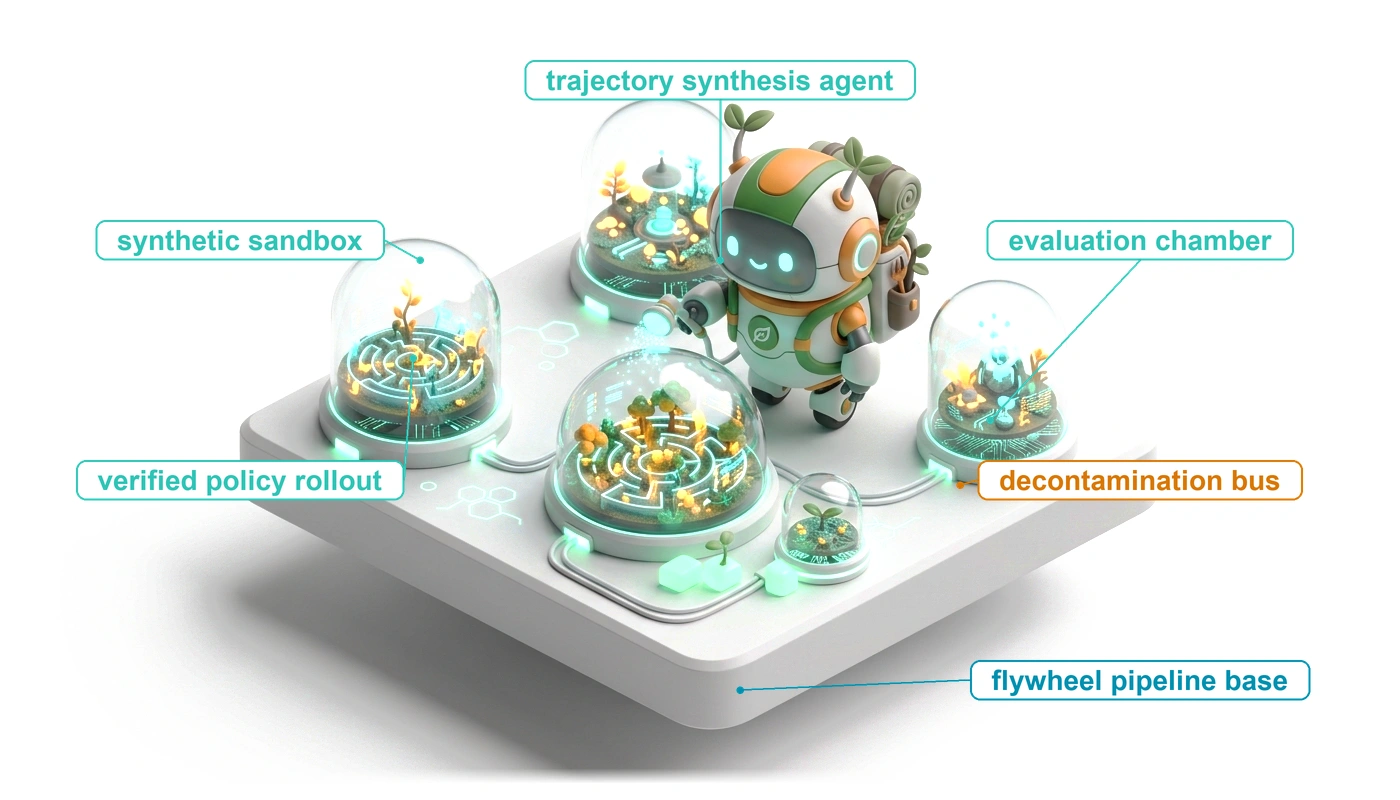
Back to top