Milestone 06: MLPerf to Generative Serving (2018)
Optimization Milestone | Difficulty: ●●●● | Time: 1–2 hours | Prerequisites: Modules 01–04, 06, 07, 09, and 11–19
- The systematic optimization workflow: measure, optimize, validate, repeat
- Why profiling before optimizing beats heroic rewrites
- How to distinguish modeled storage savings, measured accuracy, and measured latency
Overview
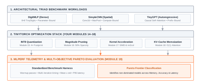
This is the Optimization Milestone: the third act of the historical arc. The Foundation Milestones proved your training loop learns. The Architecture Milestones proved your layers match real data. This one proves your optimization stack (the Profiler in Module 14, Quantization in Module 15, Compression in Module 16, Acceleration in Module 17, KV-Cache in Module 18, and Benchmarking in Module 19) can systematically evaluate and optimize the entire Architectural Triad you built across the curriculum:
- DigitMLP (Milestone 03): Dense, parameter-bound
- SimpleCNN (the Milestone 04 architecture, untrained here): Spatial, compute-bound
- TinyGPT (the Milestone 05 architecture, untrained here): Autoregressive, memory-bandwidth and prefix-bound
By 2022, ML research was sprinting while real-time interactive deployment was struggling. Generative transformers like GPT-3 and ChatGPT placed massive pressure on inference serving systems. Teams faced models too slow and expensive to serve interactively, and vendor benchmark numbers used varying datasets, batch sizes, and accuracy floors.
MLPerf established standardized evaluation: one protocol, one accuracy floor, and one set of reference models across CPUs, GPUs, and custom accelerators. Optimization transitioned from an afterthought to the discipline that decides who ships.
In this milestone, you benchmark the complete architectural triad across your optimization stack, map the Pareto frontier of non-dominated configurations, render a terminal trade-off curve, and diagnose why different neural architectures face fundamentally asymmetric hardware bottlenecks.
What You’ll Recreate
A complete MLPerf-style telemetry and optimization pipeline:
- The Architectural Triad Optimization Olympics (
01_optimization_olympics.py): profile, quantize, prune, accelerate, and cache across MLP, CNN, and TinyGPT architectures to compute the multi-dimensional Pareto frontier. - Autoregressive Generation Speedup (
02_generation_speedup.py): rigorous token-by-token logit equivalence verification and prefix replay acceleration via KV-cache memoization.
Prerequisites
Table 1 lists the modules you need to have completed before starting.
| Module | Component | What It Provides |
|---|---|---|
| 01–04, 06, 07 | Foundation | Models, loss, autograd, and the optimizer that trains the baseline (the script runs its own training loop, so Modules 05 and 08 are not required) |
| 09 | Convolutions | YOUR Conv2d for the CNN division and the reference Module 17’s im2col_conv2d is checked against |
| 11–13 | Embeddings, Attention & GPT | TinyGPT architecture for autoregressive evaluation (it runs on token IDs, so Module 10 is not required) |
| 14 | Profiling | YOUR measurement and bottleneck identification |
| 15 | Quantization | YOUR INT8/FP16 weight quantization implementations |
| 16 | Compression | YOUR magnitude pruning techniques |
| 17 | Acceleration | YOUR vectorized operations |
| 18 | Memoization | YOUR KV-cache for generation |
| 19 | Benchmarking | YOUR standardized benchmark reports and Pareto frontier |
Running the Milestone
Before running, ensure you have completed Modules 01–04, 06, 07, 09, and 11–19. You can check your progress:
tito module statustito milestone run 06 # both required parts, in order
tito milestone run 06 --part 1 # run the Architectural Triad Optimization Olympics
tito milestone run 06 --part 2 # speed up transformer generation with the KV cacheEach --part run records only that part; Milestone 06 completes once both have passed.
Pass Gates
Part 1 checks that each optimization is correct before it reports any speed or size. It stops with a teaching message at the first gate that fails:
- Loss: YOUR
CrossEntropyLosson the baseline’s first training batch matches a NumPy computation. - Profiler: YOUR parameter and FLOP counts match counts derived from the layer shapes (2,410 parameters; 4,736 FLOPs at \(2 \cdot \text{in} \cdot \text{out}\) per
Linear), and the measured latency is positive and finite. - Baseline: the FP32
DigitMLPtrained with YOUR optimizer reaches at least 80% test accuracy. - Quantization: every parameter becomes real INT8 codes (integers in \([-128, 127]\)) that dequantize back to the weights, and INT8 accuracy stays within 3 points of the baseline.
- Pruning: the pruned model’s zero fraction lands at 50% ± 2%.
- GPT behavior: before the GPT is cached, timed, or quantized, its logits vary across tokens and positions, changing later tokens never moves earlier predictions, a single token repeated along the sequence gives different predictions at different positions, and changing earlier tokens does.
- KV cache: the cache returns what was stored,
resetrewinds it, and cached logits match recomputed logits to within \(10^{-4}\). - Kernels:
vectorized_matmulmatches a loop reference andim2col_conv2dmatches YOURConv2d, each to within \(10^{-3}\). - Benchmarking: YOUR
BenchmarkResultstatistics andpareto_frontiermatch hand-worked fixtures before they score any candidate, and each measured latency summary is consistent (minimum no larger than mean and median, which are no larger than maximum).
INT8 byte counts are read from the code arrays YOUR quantizer returned (one byte per code plus a scale and zero point per tensor), not from the compression ratio it reports. Timings are reported as measured: a ratio below 1 prints as “slower”, and only a speedup of 2× or more gets a ⚡. Part 2 first applies the same GPT behavior check (logits vary, no position reads later tokens, every position reads earlier ones), since an all-zero model would pass the cache comparison trivially. It then passes when cached decoding reproduces the recomputed logits at every position.
Expected Results
Part 1: Three MLPerf Benchmark Divisions
MLPerf organizes workloads into distinct benchmark divisions because different machine learning domains face fundamentally different systems constraints. You evaluate the three architectures in their own divisions:
Division 1: Edge & Embedded Inference: DigitMLP (Dense)
Primary Bottleneck: Dense weight memory capacity (SRAM/Flash storage footprint).
Table 2 reports the candidates for DigitMLP evaluated on held-out TinyDigits test data.
tito computes the Status column from your own run’s frontier.
| Candidate | Memory | Accuracy | Latency | Status |
|---|---|---|---|---|
| Baseline FP32 | 9,640 B | 86.5% | 0.023 ms | ● Dominated |
| INT8 Quantized | 2,442 B | 86.5% | 0.023 ms | ★ Pareto |
| 50% Pruned | 9,640 B | 86.0% | 0.027 ms | ● Dominated |
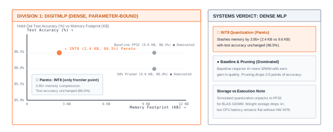
Division 1 Takeaway: Fully connected feed-forward models are memory-bound by weight parameters. INT8 Quantization shrinks weight memory by \(3.95\times\) (from 9,640 B to 2,442 B, scale and zero-point metadata included) with no accuracy change in this run (86.5% on the held-out test set), which puts it on the measured frontier. Baseline FP32 is dominated in this run because INT8 matched its accuracy with less weight memory. Unstructured pruning zeros 50% of the weights with minimal accuracy degradation (86.0%), but requires sparse index storage (such as CSR) to translate sparsity into physical memory reductions.
Quantizing model weights from FP32 to INT8 achieves a modeled \(4.0\times\) reduction in weight memory and memory bandwidth. However, pure Python and NumPy run simulated quantization: weights are stored in 8-bit precision but dequantized back to FP32 at runtime to execute standard BLAS GEMM.
Without dedicated hardware execution units (such as NVIDIA DP4A / Tensor Cores, Apple Neural Engine, or ARM NEON dot-product instructions), CPU inference latency remains flat or slightly slower. Real-world systems engineers strictly separate storage and bandwidth gains from compute execution speedups.
Division 2: Spatial Vision & Compute: SimpleCNN (Spatial)
Primary Bottleneck: 2D sliding convolution loops and spatial feature extraction throughput.
Table 3 reports the candidates for SimpleCNN evaluated via Module 19’s Benchmark harness. The CNN here is untrained, so there is no accuracy to report. Quality is agreement with the FP32 model’s outputs (cosine similarity of the output logits on test samples), not accuracy.
tito computes the Status column from your own run’s frontier.
| Candidate | Memory | Agreement w/ FP32 | Latency | Status |
|---|---|---|---|---|
| Baseline FP32 | 2,664 B | reference | 1.48 ms | ★ Pareto |
| INT8 Quantized | 714 B | 99.99% | 1.33 ms | ★ Pareto |
| 50% Pruned | 2,664 B | 95.05% | 1.31 ms | ● Dominated |
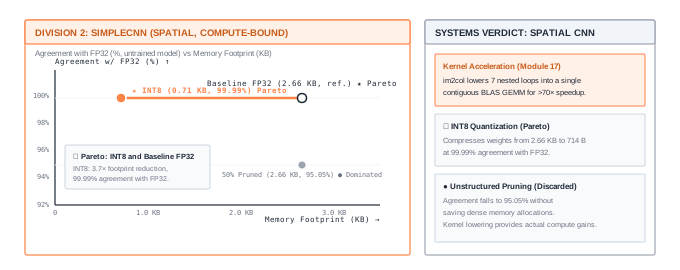
Division 2 Takeaway: Convolutional networks have a compact parameter footprint (2.66 KB) but high computational intensity across spatial loops. In this run, Baseline FP32 and INT8 Quantization form the measured frontier: INT8 shrinks storage about \(3.7\times\) (down to 714 B) while its outputs still agree with the FP32 model’s at about 99.99% cosine similarity, and 50% pruning drops agreement to about 95% without saving memory under dense array storage.
While quantization addresses model storage, Module 17’s kernel acceleration attacks the spatial convolution compute bottleneck. By unfolding the input feature map via im2col into a 2D patch matrix, the 7 nested Python loops of standard Conv2d are lowered into a single vectorized matrix multiplication (vectorized_matmul), delivering an empirical \(>70\times\) speedup (1.83 ms down to 0.02 ms in forward execution)!
Division 3: Generative LLM Serving: TinyGPT (Autoregressive)
Primary Bottleneck: \(O(N^2)\) causal prefix recomputation and DRAM weight streaming during token decoding.
Table 4 reports the serving strategies for TinyGPT across 10 repeated generation trials wrapped in Module 19’s BenchmarkResult. This GPT is untrained too, so quality is agreement with the FP32 model’s logits, not accuracy.
tito computes the Status column from your own run’s frontier.
| Serving Strategy | Memory | Agreement w/ FP32 | Latency | Status |
|---|---|---|---|---|
| Baseline FP32 (Recompute) | 113,152 B | reference | 5.44 ms | ★ Pareto |
| INT8 Quantized (Recompute) | 28,584 B | 99.97% | 5.02 ms | ★ Pareto |
| KV-Cached (Mod 18) | 129,536 B | 100.00% | 3.71 ms | ★ Pareto |
| Full Stack (Quant+Cache) | 44,968 B | 99.97% | 3.81 ms | ★ Pareto |
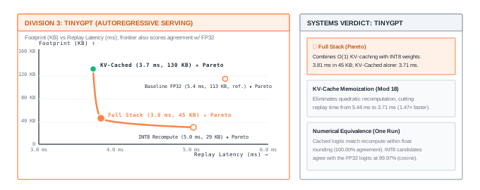
Division 3 Takeaway: Autoregressive generation is throttled by causal attention history and weight streaming. KV-Cache memoization skips quadratic prefix reprocessing (in this run, replay latency fell from 5.44 ms to 3.71 ms, about \(1.5\times\)), and its logits match recompute to within floating-point rounding. INT8 quantization shrinks weight memory about \(3.96\times\) (113,152 B to 28,584 B, scale and zero-point metadata included). Combined (Full Stack), latency is 3.81 ms, close to KV-cache alone (3.71 ms), at 45 KB including the cache. In this run all four strategies sit on the measured frontier, because each trades latency, memory, and agreement differently; none is best on all three.
Part 1 (continued): Kernel Acceleration & Systems Speedups
Beyond model compression (quantization and pruning), Milestone 06 evaluates the systems-level kernel optimizations you authored in Modules 17 and 18. Each optimization attacks a distinct computational bottleneck:
- Baseline (3 Nested Interpreter Loops): 5.17 ms
- Vectorized (NumPy BLAS call): 0.02 ms
- Measured ratio: 248.5× faster ⚡
- Mechanism:
vectorized_matmulreplaces interpreter loop overhead with one BLAS call, which runs contiguous vector instructions.
- Baseline (YOUR Conv2d forward): 1.83 ms
- Lowered (im2col Patch GEMM): 0.02 ms
- Measured ratio: 76.9× faster ⚡
- Mechanism:
im2col_conv2dlowers sliding spatial convolution loops into a single contiguous BLAS matrix multiplication.
- Baseline (full prefix recomputed each step): 4.59 ms
- KV-cached (one new token per step): 3.68 ms
- Measured ratio: 1.25× faster
- Mechanism:
KVCachememoizes previous Key/Value attention tensors, so each step projects only the new token; attention still reads all \(t\) cached positions, so a step costs \(O(t)\) instead of \(O(t^2)\). Cached and uncached logits match within float rounding. On small workloads the cache can be slower, which is why the speedup is measured, not assumed.
Table 5 summarizes the measured ratios across these three workloads.
| Kernel / Workload | Baseline (Unoptimized) | Candidate (TinyTorch) | Measured Ratio |
|---|---|---|---|
| Dense GEMM (32×32) | 5.17 ms (loops) | 0.02 ms (BLAS) | 248.5× faster ⚡ |
| 2D Conv (4-ch, 8×8) | 1.83 ms (Conv2d) | 0.02 ms (im2col) | 76.9× faster ⚡ |
| Autoregressive Decode (16 tokens) | 4.59 ms (recompute) | 3.68 ms (cached) | 1.25× faster |
Part 2: Autoregressive Generation Speedup
Table 6 shows median total prefix-replay time with and without the KV cache.
| Mode | Prefix-replay time | Speed ratio |
|---|---|---|
| Without KV-Cache | Measured baseline | 1× |
| With KV-Cache | Measured cached time | Baseline time / cached time |
Small workloads can be slower with caching. Output agreement is required; speedup is an experimental result. On our benchmark run, cached replay delivered a 1.44× speedup over full causal prefix recomputation.
The Aha Moment: Systematic Beats Heroic
The wrong way (heroic optimization):
"It's too slow! Let me rewrite everything in C++!"
"Memory is too high! Let me redesign the architecture!"
"KV-cache sounds complex! Let me try CUDA kernels first!"
Result: weeks of work, marginal gains, introduced bugs.
The right way (systematic optimization):
1. MEASURE:   Record baseline accuracy, dense bytes, and latency
2. OPTIMIZE:  Create rounded and pruned candidates independently
3. VALIDATE:  Measure each candidate on the same held-out data
4. REPEAT:    Keep useful changes and investigate remaining costs
Result: a comparison that reveals whether each change meets your accuracy and performance requirements.
This is what separates ML researchers from ML engineers:
- YOUR Profiler (Module 14) identifies real bottlenecks (not assumed ones)
- YOUR Quantization (Module 15) exposes rounding error and modeled packed storage
- YOUR Pruning (Module 16) changes the zero fraction without shrinking dense arrays
- YOUR KV-Cache (Module 18) avoids recomputing past keys and values
The full loop (measure, optimize, validate) runs on YOUR tools, not someone else’s library.
Your Code Powers This
Every optimization tool you exercise here comes from YOUR implementations:
Table 7 names the TinyTorch components that power this milestone.
| Component | Your Module | What It Does |
|---|---|---|
Profiler |
Module 14 | YOUR measurement and bottleneck identification |
| Quantization tools | Module 15 | Weight rounding and storage estimates |
| Pruning tools | Module 16 | Weight masking and sparsity measurement |
Vectorization & im2col_conv2d |
Module 17 | Replacing nested convolution loops with lowered BLAS GEMM kernels (>70× speedup) |
KVCache |
Module 18 | YOUR key-value caching for generation |
Benchmark & pareto_frontier |
Module 19 | YOUR standardized reporting and multi-objective Pareto frontier |
The measured candidates still execute dense float32 operations. Packed storage and sparse execution require additional implementations.
Historical Context
Before MLPerf, comparing ML systems was guesswork. Vendors picked their own datasets, batch sizes, and accuracy targets, then claimed wins. MLPerf forced a common protocol: same models, same data, same accuracy floor: so a “2× faster” claim could finally be checked instead of believed.
That protocol marks the moment ML engineering became as load-bearing as ML research. Building a model is step one. Shipping it inside a latency budget, on hardware your users actually own, is where production value lives, and where careers are made.
Systems Insights: Asymmetric Architectural Bottlenecks
The most profound lesson of MLPerf is that optimization is not one-size-fits-all. Each architecture in the triad is constrained by a fundamentally different physical bottleneck:
- DigitMLP (1986): Dense, Parameter-Bound:
- The Bottleneck: Over 99% of its memory footprint resides in fully connected weight matrices (\(64 \times 32\) and \(32 \times 10\)). Computational FLOPs are negligible (\(< 5{,}000\)).
- The Winning Optimization: INT8 Quantization (Module 15) compresses weight storage by \(3.95\times\), with no accuracy change in our run (86.5% before and after). Pruning (Module 16) zeros half the weights, but dense array storage is unchanged without sparse index encodings (e.g., CSR).
- SimpleCNN (1998): Spatial, Compute-Bound:
- The Bottleneck: Parameter memory is minuscule (2.6 KB), but sliding 2D convolution windows across feature maps requires thousands of nested loop iterations. The model is compute-bound and Python loop overhead dominates.
- The Winning Optimization: Vectorization & SIMD (Module 17) transforms spatial convolutions into matrix operations (im2col / GEMM), removing interpreter overhead and handing the arithmetic to an optimized BLAS library.
- TinyGPT (2017–2022): Autoregressive, Memory-Bandwidth & Prefix-Bound:
- The Bottleneck: Autoregressive token-by-token generation re-evaluates self-attention keys and values over an ever-expanding prefix. Naive generation scales as \(O(N^2)\) in total computation, repeatedly re-reading and re-projecting past tokens through memory.
- The Winning Optimization: KV-Cache Memoization (Module 18) caches prior key and value tensors, so each new token projects only itself while attention still reads the whole cached prefix (\(O(t)\) per step instead of \(O(t^2)\)). Combined with INT8 quantization to cut weight memory traffic, these are two techniques production LLM serving commonly combines.
Read why
The companion book’s chapter Synthesis III: The MLPerf Optimization Olympics covers this milestone’s scoring and what each measurement can and cannot show. Read it in TinyTorch: From Tensors to Transformers (PDF) after you have run the milestone.
What’s Next
With Milestone 06, the optimization arc is complete. You have:
- Built every core component (Modules 01–13)
- Implemented and measured optimization techniques (Modules 14–19)
- Proven mastery across six landmark systems (Milestones 01–06)
Next, test your framework in the open-ended Capstone (Module 20: Torch Olympics), and check your Module 17 kernels against native C++ SIMD, Metal, and Triton ones in Milestone 07: Custom Kernels, with the optional extensions described in Extending TinyTorch.
Further Reading
- MLPerf: mlcommons.org
- Deep Compression: Han et al. (2015). “Deep Compression: Compressing DNNs with Pruning, Trained Quantization and Huffman Coding”
- Efficient Transformers: Tay et al. (2020). “Efficient Transformers: A Survey”