🚧 DEVELOPMENT PREVIEW - Built from dev@75c25583 • 2026-07-15 02:21 EDT • Stable version →
🧮 MLSys·im — first-principles analytical modeling for ML training and inference; model the physics before you build. 📘 The book:Vol I: Foundations · Vol II: At Scale — open access, free forever. 🛠️ Alongside the book:TinyTorch (build) · Hardware Kits (deploy) · Labs (explore) · StaffML (practice) · Lecture Slides 📬 Newsletter: ML Systems insights & updates — Subscribe →
Hello, Roofline
Five lines of code to predict whether your model is memory-bound or compute-bound.
start
beginner
Learn to use MLSys·im’s analytical roofline model to predict ML model performance on any hardware. The foundation for all ML systems reasoning.
The Question
You have a model and a GPU. Before you write any code, train anything, or rent any cloud instance — can you predict which hardware resource will be the bottleneck?
This tutorial teaches the single most important skill in ML systems: using the roofline model to answer that question in under a second.
NotePrerequisites
None. This is the starting point for all MLSys·im tutorials.
TipKey Terms for These Tutorials
If you are new to ML, here are the essential terms used throughout this tutorial series:
Term
Meaning
Model
A mathematical function with learned parameters (weights) that maps inputs to outputs — e.g., an image to a label
Parameters
The numbers a model learns during training. A “25M parameter” model stores 25 million numbers
Inference
Running a trained model on new input to get a prediction (as opposed to training, which learns the parameters)
CNN
Convolutional Neural Network — a model architecture for images (e.g., ResNet-50)
LLM
Large Language Model — a model that generates text one token (roughly one word) at a time (e.g., GPT-4, Llama-3)
FP16
16-bit floating point (“half precision”) — uses 2 bytes per parameter. ML often uses reduced precision for speed
FLOP/s
Floating-point operations per second — a measure of compute speed. TFLOP/s = trillion FLOP/s
HBM
High Bandwidth Memory — the fast DRAM attached to a GPU (e.g., HBM2e on A100, HBM3 on H100)
Batch size
How many inputs are processed together in one pass. Larger batches amortize the cost of loading weights
Identify the performance bottleneck (memory-bound vs. compute-bound) for any model-hardware pair
Predict how batch size shifts the operating point along the roofline
Interpret the ridge point as the boundary between two performance regimes
UseEngine.solve as the foundational API for all MLSys·im analyses
TipBackground: The Roofline Model
The roofline model (Williams, Waterman, and Patterson, 2009) is the foundational analytical tool for predicting hardware bottlenecks. Every accelerator has two speed limits:
Compute ceiling — how fast it can do arithmetic (measured in FLOP/s)
Memory bandwidth ceiling — how fast it can load data from memory (measured in bytes/s)
The roofline model reduces to four lines of algebra:
Your model’s arithmetic intensity (FLOPs ÷ Bytes) determines which ceiling you hit. If it is below the ridge point, you are memory-bound (starved for data). Above it, you are compute-bound (saturating the arithmetic units). This single classification drives every optimization decision downstream.
Important caveat: The roofline is an upper bound. Real performance is always below it due to scheduling overhead, memory access patterns, and imperfect utilization. Achieving 40–60% of the roofline ceiling is considered good in practice. The model’s value is not in predicting exact latency — it is in identifying the binding constraint (which resource limits you).
NoteConventions Used in These Tutorials
FLOP counting: We count one multiply-accumulate (MAC) as 1 FLOP, consistent with the MLSys Zoo constants. Industry and vendor datasheets typically count 1 MAC = 2 FLOPs. This factor of 2 shifts the ridge point: the A100’s ridge is ~156 FLOP/byte in our convention but ~312 in the 2-FLOP convention. Always check which convention a paper uses before comparing numbers.
Peak specs: We use vendor-published peak Tensor Core throughput and peak HBM bandwidth. Real sustained performance is typically 70–90% of these peaks.
Units:Q_ creates physical quantities with units (e.g., Q_("2 TB/s")). The ~ in format strings like :~.2f shows abbreviated unit names.
1. Setup
After pip install mlsysim, the import is two lines:
import mlsysimfrom mlsysim import Engine
2. Pick a Model and a GPU
Pull vetted specifications from the MLSys Zoo — no need to search datasheets.
The Engine.solve method applies the roofline model — it calculates which of the two speed limits you hit first, and returns latency, throughput, and the bottleneck classification.
# One line: model + hardware + config → performance predictionprofile = Engine.solve( model=model, hardware=hardware, batch_size=1, # Single image inference precision="fp16"# Half-precision (16-bit floating point))info(Bottleneck=profile.bottleneck, Latency=profile.latency.to('ms'), Throughput=f"{profile.throughput:.0f} images/sec")
Bottleneck:  Compute
Latency:     0.568 ms
Throughput:  1762 / second images/sec
At batch size 1, ResNet-50 performs ~4.1 GFLOP but must load ~50 MB of weights (25M params × 2 bytes). That gives an arithmetic intensity of ~82 FLOP/byte — close to the A100’s ridge point of ~156 FLOP/byte. At this operating point, the two ceilings are nearly balanced, and the bottleneck label depends on exact assumptions. The important takeaway: most of the A100’s 312 TFLOP/s is idle — you need larger batches to exploit it.
Sanity check: We can verify this with the equation from the Background. Note: we use our 1-FLOP-per-MAC convention here, so the A100’s peak is 156 TFLOP/s (the vendor-reported 312 TFLOP/s uses the 2-FLOP convention):
\(T = \max(0.025, 0.026) = 0.026\;\text{ms}\) → the two ceilings are nearly equal ✓
ResNet-50 at batch 1 sits right at the ridge point. When \(T_{\text{compute}} \approx T_{\text{memory}}\), the regime label is ambiguous — and that is the point: the ridge is a boundary, not a wall. Small differences in convention or measurement can flip the label. Engine.solve handles the convention internally, so its reported latency may differ slightly from this back-of-envelope estimate. The skill that matters is computing the ratio and knowing where you stand.
Computing arithmetic intensity from first principles: This is the skill that lets you reason about any model, not just ones in the Zoo. The formula is FLOPs ÷ Bytes. Compare two very different workloads:
ResNet-50 (batch 1): 4.1 GFLOP ÷ 50 MB = 82 FLOP/byte → near the A100 ridge (156) — balanced
LLM decode (batch 1): Each token does ~2 FLOP per parameter but loads 2 bytes per parameter = 1 FLOP/byte → deeply memory-bound (you will explore this in Tutorial 2)
When you encounter an unfamiliar model, compute this ratio first. It tells you the regime before you touch any code.
4. Sweep Batch Size: Watch the Regime Shift
Now let’s increase the batch size and see when the bottleneck changes. More images per batch means more computation per weight load — which increases arithmetic intensity.
Batch  Bottleneck        Throughput   Latency
─────────────────────────────────────────────
1         Compute   1762 / second/s  0.568 ms
4         Compute   5515 / second/s  0.725 ms
16        Compute  11799 / second/s   1.36 ms
32        Compute  14565 / second/s   2.20 ms
64        Compute  16499 / second/s   3.88 ms
128       Compute  17672 / second/s   7.24 ms
256       Compute  18323 / second/s  13.97 ms
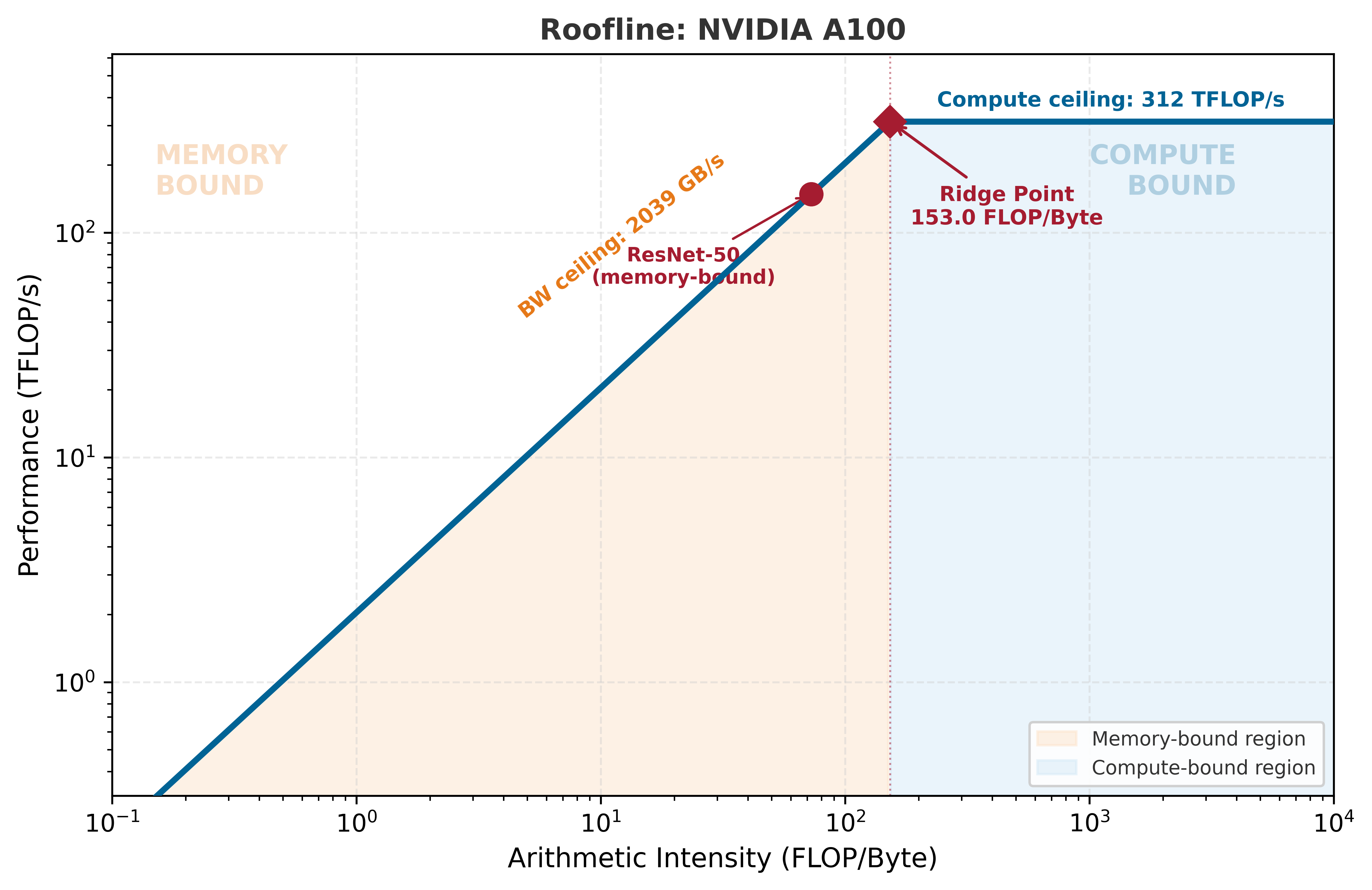
We can visualize this transition on the Roofline model. Notice where the model sits relative to the “ridge point” (the crossover between memory-bound and compute-bound regimes).
from mlsysim.viz.plots import plot_roofline# The plot_roofline function takes the hardware node and a list of workloadsfig, ax = plot_roofline(hardware, workloads=[model])
ImportantKey Insight
The roofline model lets you predict performance without running a single experiment. The answer is determined by two ratios: your workload’s arithmetic intensity and the hardware’s ridge point. Batch size is the primary knob that moves you along the roofline — at small batches you are memory-bound, at large batches compute-bound. The ridge point is the most efficient operating point. Every optimization decision starts with knowing which side of the ridge you are on.
A common mistake is selecting hardware based on peak FLOP/s alone. At batch size 1, ResNet-50 is memory-bound — the 312 TFLOP/s compute ceiling is irrelevant. A GPU with half the FLOP/s but the same bandwidth would deliver identical inference latency. Always check the regime before comparing specs.
Your Turn
CautionExercises
Exercise 1: Predict before you compute. Before running any code: will ResNet-50 at batch_size=64 be memory-bound or compute-bound on the A100? Write your answer as one of: “memory-bound” or “compute-bound”, plus one sentence of reasoning. Then verify with Engine.solve(...). Were you right? What would you need to know to predict correctly?
Exercise 2: Change the hardware. Run the same batch size sweep on the H100 (mlsysim.Hardware.Cloud.H100). The H100 has 3.2× more FLOP/s than the A100 but only 1.7× more bandwidth. How does the ridge point shift? At what batch size does the crossover happen on the H100 vs. the A100?
Exercise 3: Change the model. Replace ResNet-50 with Llama-3 8B (mlsysim.Models.Language.Llama3_8B). At batch size 1, is it memory-bound or compute-bound? Does the answer surprise you? Why do large language models behave differently from CNNs at the same batch size?
Self-check: If a model’s arithmetic intensity is 50 FLOP/byte and the hardware’s ridge point is 156 FLOP/byte, is the model memory-bound or compute-bound?
Key Takeaways
TipSummary
The roofline model predicts performance by comparing arithmetic intensity to the hardware’s ridge point
Memory-bound means the GPU is waiting for data; compute-bound means it is saturating arithmetic units
Batch size is the primary knob for shifting between regimes — larger batches increase arithmetic intensity
The ridge point (\(\text{Peak FLOP/s} \div \text{Peak BW}\)) is the crossover — the most efficient operating point
Engine.solve is the foundational API: model + hardware + config → bottleneck, latency, throughput
Next Steps
The Memory Wall — Discover why upgrading from A100 to H100 doesn’t give the speedup you expect
Two Phases, One Request — Learn why LLM serving has two different bottlenecks in the same request
Silicon Zoo — Browse all vetted hardware specifications
Math Foundations — The complete equations behind the roofline model