Sustainable AI
Purpose
Why does energy consumption determine what machine learning systems can exist, not just what they cost to operate?
Power is not merely an operational expense but a hard physical constraint that limits what can be built. A data center has a fixed power budget determined by its electrical infrastructure and cooling capacity; exceeding that budget is not expensive but impossible. Training runs that require more power than available cannot happen regardless of budget. Deployment locations are constrained by grid capacity and cooling feasibility, not just real estate prices. At frontier scale, the question shifts from “can we afford this” to “can this physically exist”—and the answer increasingly depends on energy efficiency rather than algorithmic capability. The organizations pushing machine learning forward are those that treat energy as a first-class engineering constraint alongside accuracy and latency, because sustainability is not about virtue but about the physics that determines which ambitious systems can actually be built and operated (Lam et al. 2023; Kurth et al. 2023).
Lam, R., A. Sanchez-Gonzalez, M. Willson, P. Wirnsberger, M. Fortunato, F. Alet, S. Ravuri, et al. 2023. “Learning Skillful Medium-Range Global Weather Forecasting.” Science 382 (6677): 1416–21. https://doi.org/10.1126/science.adi2336.
Kurth, T., S. Subramanian, P. Harrington, J. Pathak, M. Mardani, D. Hall, A. Miele, K. Kashinath, and A. Anandkumar. 2023. “FourCastNet: Accelerating Global High-Resolution Weather Forecasting Using Adaptive Fourier Neural Operators.” Proceedings of the Platform for Advanced Scientific Computing Conference, 1–11. https://doi.org/10.1145/3592979.3593412.
Learning Objectives
- Explain the sustainability paradox where AI compute growth outpaces hardware efficiency gains
- Analyze how Jevons Paradox causes efficiency improvements to increase total resource consumption
- Calculate Power Usage Effectiveness (PUE) and lifecycle carbon footprints across training, inference, and manufacturing, differentiating operational emissions from embodied carbon
- Analyze geographic and temporal factors affecting carbon intensity and apply these insights to workload scheduling decisions
- Evaluate algorithmic optimizations (pruning, quantization, knowledge distillation) and edge deployment for accuracy-energy trade-offs and lifecycle sustainability
- Design carbon-aware scheduling that uses renewable energy and grid intensity to cut emissions 50–80 percent while meeting performance requirements
- Critique carbon offsets vs. actual emissions reductions and synthesize multi-layer plans integrating algorithmic, infrastructure, and policy levers
This chapter’s position in the book’s organizing framework, the fleet stack, clarifies why energy and environmental constraints are not external concerns but physical limits that bound what the entire system can achieve.
Systems Perspective 1.1: Fleet stack connection
Sustainability is the final component of the Governance Layer. Security protects against adversaries; Robustness protects against operational chaos; Sustainability protects against resource exhaustion. A system that exceeds its energy budget or cannot be powered by the available grid is operationally failed in the same sense as one that crashes. Sustainability engineering ensures that the fleet continues to operate within its long-run energy and carbon constraints.
The Energy Ceiling
When an engineer optimizes a database query to save 100 milliseconds, it is considered standard performance tuning. When that same query is executed billions of times a day across a global data center, however, that 100-millisecond savings translates to megawatts of electrical power and tons of avoided carbon emissions (Lacoste et al. 2019). Sustainable AI ceases to be a theoretical ethical concern once we recognize that power density is the absolute physical ceiling on data center computational capacity; energy is the ultimate currency of machine learning.1
Lacoste, Alexandre, Alexandra Luccioni, Victor Schmidt, and Thomas Dandres. 2019. “Quantifying the Carbon Emissions of Machine Learning.” arXiv Preprint arXiv:1910.09700.
1 Joule: The SI unit of energy (1 J = 1 Watt-second). To ground the scale of the fleet: a single A100 GPU at peak load consumes ~400 Joules every second. Large-model training runs are measured in billions to trillions of joules, so small per-operation inefficiencies scale into facility-level energy demand.
Security (Security & Privacy) protects ML systems from adversarial threats. Robustness (Robust AI) ensures they perform reliably under distribution shift. This chapter addresses a third operational concern that determines long-term viability: the resource constraints that govern whether systems remain economically and environmentally sustainable at scale.
Contemporary machine learning applications operate at industrial scales, with environmental impact now comparable to established heavy industries. Training a single frontier AI model can consume as much electricity as roughly 122 US homes do in an entire year. The exponential growth trajectory of computational demands outpaces efficiency improvements in underlying hardware by orders of magnitude, establishing the sustainability paradox in artificial intelligence (Sevilla et al. 2022). This chapter formalizes these constraints into an engineering discipline: Sustainable AI.
Sevilla, J., L. Heim, A. Ho, T. Besiroglu, M. Hobbhahn, and P. Villalobos. 2022. “Compute Trends Across Three Eras of Machine Learning.” 2022 International Joint Conference on Neural Networks (IJCNN) 2202.05924: 1–8. https://doi.org/10.1109/ijcnn55064.2022.9891914.
Definition 1.1: Sustainable AI
Sustainable AI is the systems engineering practice of measuring and optimizing the full environmental cost of ML systems (energy, water, and embodied carbon across training, inference, and hardware manufacturing) and incorporating those costs as explicit constraints in architecture decisions alongside performance and accuracy objectives (Lannelongue et al. 2021).
- Significance (quantitative): Training GPT-3 consumed approximately 1,287 MWh of energy (Li 2020), equivalent to roughly 122 US household-years of electricity. Fine-tuning a pretrained model on domain data consumes roughly 1–5 percent of full training cost, making transfer learning a 20–100\(\times\) more energy-efficient path to the same capability. At inference scale, a 175B-parameter model serving 10M queries/day at 100 ms per query can consume more cumulative energy in months of production service than its training, making inference optimization the dominant sustainability lever at production scale.
- Distinction (durable): Unlike corporate sustainability reporting (which aggregates energy usage into annual CO2 disclosures), sustainable AI engineering operates at the individual workload level—selecting hardware based on FLOP/watt efficiency, scheduling training during periods of high renewable availability, and choosing model architectures that minimize inference FLOPs rather than simply maximizing accuracy.
- Common pitfall: A frequent misconception is that switching to renewable energy solves the sustainability problem. For hardware-intensive ML, embodied carbon (the carbon emitted manufacturing the chips, servers, and cooling equipment before they ever run a training job) often equals or exceeds operational carbon; over 50 percent of an edge device’s lifecycle carbon can come from manufacturing, making hardware longevity and utilization rate as important as energy source.
Li, C. 2020. Estimating the Training Cost of GPT-3.
Lannelongue, Loı̈c, Jason Grealey, and Michael Inouye. 2021. “Green Algorithms: Quantifying the Carbon Footprint of Computation.” Advanced Science 8 (12): 2100707. https://doi.org/10.1002/advs.202100707.
Jones, N. P., M. Johnson, and C. Montgomery. 2021. “The Environmental Impact of Data Centers: Challenges and Sustainable Solutions.” Energy Rep. 7: 4381–92.
The environmental impact of AI systems spans the complete lifecycle: from semiconductor manufacturing and data center construction to model training, inference deployment, and electronic waste (Jones et al. 2021). Treating this full lifecycle as an engineering problem rather than a corporate responsibility exercise transforms sustainability from a vague objective into a measurable engineering requirement. Before we can optimize this massive footprint, however, we must ground our intuition by calculating the raw physical energy required to produce frontier machine intelligence.
Checkpoint 1.1: The energy of intelligence
A 175B parameter model requires approximately \(3.14 \times 10^{23}\) FLOPs to train. Assuming a data center PUE of 1.1 and an end-to-end realized training efficiency of 50 GFLOPs/Watt:
- Calculate the total energy consumption in megawatt-hours (MWh).
- If the average US household consumes 10.6 MWh per year, how many “household-years” does this single training run represent?
- Discuss whether this metric captures the true environmental cost, considering the difference between energy consumption (MWh) and carbon intensity (g CO2/kWh).
The measurement, modeling, and mitigation frameworks presented in this chapter represent essential engineering competencies alongside traditional performance optimization. Mastering them requires understanding the scale of the problem, the physics that constrain solutions, and the system-level interventions that move the needle.
The scale of environmental impact
The numbers become visceral when translated into familiar physical quantities. To appreciate the scale of the problem, translate a single frontier training run into emissions and a familiar travel comparison.
Napkin Math 1.1: The carbon cost of training
Problem: A team trains a large model (GPT-3 size) consuming 1,287 MWh. How much CO2 is emitted, and how does that compare to a trans-Atlantic flight?
Math:
- Energy: 1,287 MWh = 1,287,000 kWh.
- Carbon intensity (US average): \(\approx\) 0.429 kg CO\(_2\)/kWh.
- Total Emissions: \(1,287,000 \times 0.429 \approx\) 552,123 kg CO\(_2\).
- Comparison:
- One passenger, NY to London (round trip): \(\approx 1,000 \text{ kg CO}_2\).
- Ratio: 552,123 / 1,000 = 552 flights.
Systems insight: A single training run emits as much carbon as hundreds of trans-Atlantic passenger round trips. Optimization matters. Moving this job to a hydro-powered region (0.02 kg/kWh) would reduce emissions by 21\(\times\) to about 25 passenger round trips.
That arithmetic shows the carbon cost of one run; at frontier scale, the next constraint is whether enough power can be delivered to the cluster at all.
Lighthouse 1.1: Archetype A (GPT-4/Llama-3): The energy wall
Archetype A (GPT-4) is the primary driver of the industry’s exponential energy growth. A single 25,000-GPU cluster drawing 700 W per chip requires 17.5 MW of accelerator power before server, network, and cooling overhead. The constraint is physical, not financial: it is a Grid Capacity problem. Organizations operating Archetype A models are increasingly forced to build their own power infrastructure or relocate to regions with excess renewable energy, making Carbon-Aware Scheduling and Geographic Optimization as critical as learning rate tuning.
AI systems consume resources at industrial scales that rival traditional heavy industries.
Napkin Math 1.2: Automated carbon-aware scheduling (Tier 3 optimizer)
Problem: A team is planning a large training run requiring 10,000 MWh of energy, choosing between three regions with different electricity prices and carbon intensities. With an internal carbon tax of USD 100/tonne, which region minimizes the true Total Cost of Ownership (TCO)?
Solution: We invoke the PlacementOptimizer to synthesize grid carbon intensity, regional electricity rates, and the carbon tax into a single optimization objective.
Result: The optimizer evaluates the design space and selects the global minimum:
- Optimal Region: Quebec
- Total Projected Cost: USD 0.79 million (Including carbon penalty)
Systems insight: In a pure energy-cost-only model, engineers might choose the region with the lowest raw electricity rate. However, once a carbon tax is introduced, the Externalities Wall becomes a first-class economic constraint. The optimizer proves that the hydro-powered grid in Quebec is the most cost-effective choice, as the massive carbon savings more than offset any marginal difference in electricity pricing.
That optimization result rests on a simpler physical fact: identical energy demand produces radically different emissions depending on the grid that supplies it.
Napkin Math 1.3: The geography of carbon
Problem: A team is choosing a data center for a 10,000 MWh training run.
- Site A (Quebec): Hydropower, 20 g \(\text{CO}_2\)/kWh.
- Site B (Poland): Coal-heavy, 800 g \(\text{CO}_2\)/kWh. How does the location affect a model’s carbon footprint?
Math: Carbon = Energy \(\times\) Grid Intensity.
- Site A Emissions: 10,000,000 kWh \(\times\) 20 g = 200,000,000 g = 200 tonnes \(\text{CO}_2\).
- Site B Emissions: 10,000,000 kWh \(\times\) 800 g = 8,000,000,000 g = 8,000 tonnes \(\text{CO}_2\).
- Ratio: 8,000/200 = 40\(\times\) difference.
Systems insight: Site selection is the single most effective tool for sustainable AI. A 40\(\times\) difference in carbon emissions is larger than any possible algorithmic speedup. In the Machine Learning Fleet, Carbon-Aware Scheduling (moving nonurgent jobs to low-carbon regions or hours) is a first-class operational competency. Efficiency extends beyond FLOPs to the Carbon-Intensity of those FLOPs.
Training a single large language model consumes thousands of megawatt-hours of electricity, equivalent to powering hundreds of households for months.2 IEA projects global data-center electricity consumption to reach about 945 TWh by 2030, just under 3 percent of global electricity demand, with AI-accelerated servers driving much of the growth.3 Computational demands increased 350,000\(\times\) from 2012 to 2019 (Schwartz et al. 2020), while hardware efficiency improved at a far slower rate, creating an unsustainable growth trajectory.
2 Household Energy Baseline: The average U.S. household consumes 10,500 kWh annually. GPT-3’s verified 1,287 MWh training run equals 122 households’ annual electricity, and later frontier-scale runs can require substantially more compute. This comparison anchors an otherwise abstract energy figure to physical infrastructure: a single training run draws more grid capacity than a residential neighborhood.
3 Data Center Industrial Scale: IEA’s 2025 Energy and AI analysis projects data centers to consume about 945 TWh of electricity by 2030, just under 3 percent of global electricity demand. This is an electricity-demand metric, not directly comparable to aviation or cement shares of global emissions, but it still means AI infrastructure competes for grid capacity with heavy industry: regions that cannot expand power generation cannot expand AI deployment, regardless of demand.
4 GPU Manufacturing Embodied Carbon: A single H100 GPU embodies 150–200 kg CO2 from fabrication before computing its first FLOP. Advanced-node manufacturing also requires substantial ultrapure water, specialty gases, chemicals, and high-temperature process steps. This embodied cost means that in clean-grid regions (hydro, nuclear), manufacturing emissions can rival or exceed operational carbon, making hardware longevity and circular economy reuse critical sustainability levers.
Forti, V., C. P. Baldé, R. Kuehr, and G. Bel. 2020. The Global e-Waste Monitor 2020: Quantities, Flows and the Circular Economy Potential. United Nations University/United Nations Institute for Training; Research, International Telecommunication Union,; International Solid Waste Association.
5 AI Hardware E-Waste: Global e-waste reached 53.6 million metric tons in 2019, with computing equipment contributing 15 percent. AI accelerators compound this: 3-5 year obsolescence cycles driven by rapidly advancing architectures mean that a fleet of 10,000 GPUs generates 10–20 metric tons of toxic e-waste per refresh cycle, containing lead, mercury, and cadmium requiring specialized disposal.
Beyond direct energy consumption, AI systems drive environmental impact through hardware manufacturing and resource consumption. Training and inference workloads depend on specialized processors that require rare earth metals whose extraction and processing generate pollution.4 The growing demand for AI applications accelerates electronic waste production, with global e-waste reaching 54 million metric tons annually (Forti et al. 2020; Baldé et al. 2017). AI hardware rapidly becomes obsolete due to accelerating performance requirements.5
Addressing these environmental challenges demands a coordinated response across technical, policy, and ethical dimensions to ensure AI development remains viable and responsible.
Environmental impact and ethical foundations
When training a single language model consumes electricity equivalent to hundreds of homes annually, urgent questions arise about who benefits from AI progress and who bears its ecological costs. The intersection of exponential computational demands with finite planetary resources demands that the field confront difficult choices about sustainable development pathways balancing innovation with environmental responsibility.
Environmental justice and responsible development
The environmental impact of AI creates ethical responsibilities that extend beyond technical optimization. Environmental sustainability emerges as a critical component of trustworthy AI systems, extending the responsible AI principles examined in Responsible Engineering to include ecological stewardship (Vinuesa et al. 2020). The computational resources required for AI development concentrate environmental costs on specific communities while distributing benefits unequally across global populations. Data centers consume on the order of a few percent of global electricity and substantial water for cooling (Andrae and Edler 2015; Jones 2018), often in regions where energy grids rely on fossil fuels and water resources face stress from climate change.
Vinuesa, Ricardo, Hossein Azizpour, Iolanda Leite, Madeline Balaam, Virginia Dignum, Sami Domisch, Anna Felländer, Simone Daniela Langhans, Max Tegmark, and Francesco Fuso Nerini. 2020. “The Role of Artificial Intelligence in Achieving the Sustainable Development Goals.” Nature Communications 11 (1): 233. https://doi.org/10.1038/s41467-019-14108-y.
Andrae, Anders, and Tomas Edler. 2015. “On Global Electricity Usage of Communication Technology: Trends to 2030.” Challenges 6 (1): 117–57. https://doi.org/10.3390/challe6010117.
Jones, N. 2018. “How to Stop Data Centres from Gobbling up the World’s Electricity.” Nature 561 (7722): 163–66. https://doi.org/10.1038/d41586-018-06610-y.
6 Environmental Justice in Data center Siting: Data centers gravitate toward low-cost land and electricity, which often means economically disadvantaged areas. The result is an asymmetric externality: communities hosting AI infrastructure bear water depletion, heat island effects, and grid strain, while economic benefits concentrate in distant tech hubs. For ML systems engineers, this creates a design constraint: site selection must factor in social license alongside grid carbon intensity, because community opposition can block or delay facility expansion.
Geographic concentration of environmental burden creates questions of environmental justice that align with broader responsible AI frameworks.6 Fairness considerations require examining who benefits from AI systems and who bears their risks; environmental responsibility demands understanding who pays the ecological costs of AI advancement. Communities hosting AI infrastructure bear disproportionate environmental burdens while having limited access to AI’s economic benefits, exemplifying the need to extend ethical AI frameworks beyond algorithmic fairness to encompass environmental stewardship.
Exponential growth vs. physical constraints
Exponential growth in computational demands challenges the long-term sustainability of AI training and deployment. Over the past decade, AI systems have scaled faster than any prior computing workload, with compute requirements increasing 350,000\(\times\) from 2012 to 20197 (Schwartz et al. 2020). This trend continues as machine learning systems prioritize larger models with more parameters, larger training datasets, and higher computational complexity. Sustaining this trajectory poses sustainability challenges, as hardware efficiency gains fail to keep pace with rising AI workload demands.
7 AI Compute Growth Rate: The 350,000\(\times\) increase from 2012 to 2019 implies a doubling time of approximately 4.6 months, roughly 5.3\(\times\) faster than Moore’s Law’s 2-year doubling. This divergence is the root cause of the energy wall: no physically realizable improvement in silicon efficiency can match a doubling cadence measured in months, making algorithmic efficiency and carbon-aware scheduling the only viable sustainability levers at scale.
Schwartz, R., J. Dodge, N. A. Smith, and O. Etzioni. 2020. “Green AI.” Communications of the ACM 63 (12): 54–63. https://doi.org/10.1145/3381831.
8 Moore’s Law: Gordon Moore’s 1965 observation that transistor density doubles every two years drove 60 years of “free” efficiency gains for the semiconductor industry. At 3nm process nodes, physical limits are ending this trajectory: individual atoms become the constraint. For AI sustainability, the end of Moore’s Law means that future efficiency gains must come from architectural specialization and algorithmic optimization rather than process shrinks.
9 Dennard Scaling: Robert Dennard observed in 1974 that smaller transistors could operate at constant power density by reducing voltage proportionally. This ended around 2005 when leakage current made further voltage reduction impractical. The consequence for AI sustainability is direct: without Dennard scaling, each new process node no longer delivers proportional power savings, forcing the shift to specialized accelerators—GPUs and Tensor Processing Units (TPUs)—that achieve efficiency through architectural parallelism rather than transistor physics.
Historically, computational efficiency improved with advances in semiconductor technology. Moore’s Law predicted that the number of transistors on a chip would double approximately every two years, leading to continuous improvements in processing power and energy efficiency.8 However, Moore’s Law is now reaching core physical limits, making further transistor scaling difficult and costly. Dennard scaling, which once ensured that smaller transistors would operate at lower power levels, has also ended, leading to stagnation in energy efficiency improvements per transistor.9
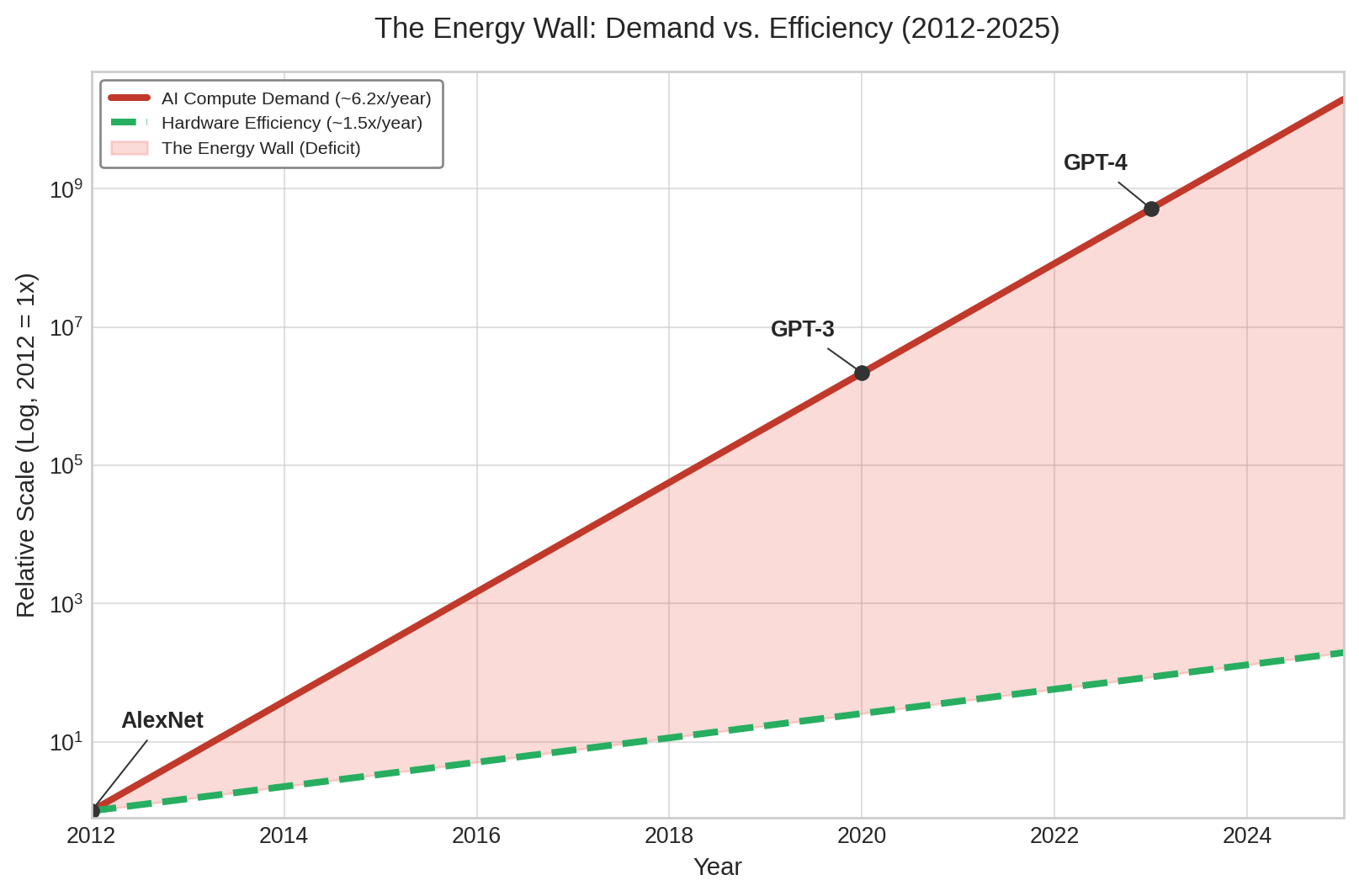
While AI models continue to scale in size and capability, the hardware running these models no longer improves at the same exponential rate. As Figure 1 illustrates, this growing divergence between computational demand and hardware efficiency creates an unsustainable trajectory where AI consumes ever-increasing amounts of energy. This technical reality underscores why sustainable AI development requires coordinated action across the entire systems stack, from individual algorithmic choices to infrastructure design and policy frameworks.
To make the uncertainty visible, Figure 2 shows high-growth sensitivity scenarios for data center electricity usage rather than the IEA baseline forecast above. The spread between best, expected, and worst cases illustrates how strongly the outcome depends on efficiency improvements and demand growth assumptions.

The energy wall: Divergent scaling
Figure 1 framed the energy wall as a divergence between compute demand and silicon efficiency. This section reframes the same divergence against a different ceiling, the physical energy infrastructure (battery density and grid efficiency), to show that the wall persists even if every accelerator hit its theoretical efficiency limit. AI sustainability presents a unique engineering challenge because it is a race between two fundamentally different physics: the exponential scaling of logic and the linear scaling of energy infrastructure.
As Figure 3 shows, AI compute grew ~350,000\(\times\) over the 2012–2019 period cited above while battery density and grid efficiency improve at only ~2–5 percent annually.

While AI logic follows the “iron law” of software optimization, energy follows the laws of chemistry and thermodynamics. Over the same seven-year interval, battery energy density would improve by only ~41 percent at a 5 percent annual rate, and grid efficiency by ~15 percent at a 2 percent annual rate. The 248,738\(\times\) gap between these curves is the Sustainability Wall—the point where we can no longer “buy our way out” of the efficiency problem with more power.
Data center grid dynamics
Sustainable AI requires looking beyond the server rack to the Electrical Grid Interface. Traditional data centers are “Steady-State” loads; they pull constant power 24/7. ML training clusters, however, are Transient Loads.
The power ramp and grid stability
As discussed in Power delivery, a 10,000-GPU cluster can swing its load by 5–10 megawatts in milliseconds during an AllReduce synchronization step. For an electrical utility, this is a noise event. When thousands of GPUs suddenly stop computing to wait for the network, they cause a voltage spike on the grid; when they resume, they cause a voltage sag. Managing these transients requires Energy Buffering: using on-site battery arrays or massive capacitors to smooth the training iterations, ensuring the ML Fleet does not destabilize the local municipal power grid.
Heat reuse: Turning waste into fuel
A data center is physically a system that converts high-quality energy (electricity) into low-quality energy (waste heat). In a sustainable fleet, this heat is not exhausted into the atmosphere but harvested. * District Heating: Modern facilities in Nordic regions (for example, Meta’s Odense facility) pipe waste heat into local municipal heating systems, providing enough thermal energy to warm thousands of homes. * Industrial Coupling: Using low-grade waste heat (~45°C) for greenhouse climate control or water desalination.
By treating heat as a byproduct rather than a pollutant, the fleet moves toward a circular energy economy10 (Un and Forum 2019).
10 PUE (Power Usage Effectiveness): In the early 2000s, PUE values of 2.0-2.5 were common, meaning more power went to cooling than to computing (Grid 2007). Google’s 2009 disclosure of PUE 1.21 proved that free-air cooling could halve data center overhead. The shift from PUE to CUE (Carbon Usage Effectiveness) and WUE (Water Usage Effectiveness) reflects a systems-level insight: optimizing watts alone is insufficient when water and carbon constraints bind independently.
Grid, The Green. 2007. Green Grid Data Center Power Efficiency Metrics: PUE and DCIE. The Green Grid.
Un, and World Economic Forum. 2019. A New Circular Vision for Electronics, Time for a Global Reboot. PACE - Platform for Accelerating the Circular Economy.
11 GPT-3 Energy Scale: GPT-3’s 1,287 MWh training cost translates to roughly $130,000 in US electricity and 552 metric tons of CO2 at average grid intensity. The energy-per-parameter ratio of approximately 7.35 MWh per billion parameters reveals the co-design opportunity: optimized architectures using mixed precision and sparsity achieve sub-1 MWh per billion parameters, a several-fold efficiency gain that compounds across frontier-scale training runs.
Maslej, Nestor, Loredana Fattorini, Erik Brynjolfsson, John Etchemendy, Katrina Ligett, Terah Lyons, James Manyika, et al. 2023. “Artificial Intelligence Index Report 2023.” ArXiv Preprint abs/2310.03715.
12 Training Communication Overhead: Distributed training adds 15–30 percent energy overhead beyond raw computation due to gradient synchronization and checkpointing across nodes. For frontier models requiring thousands of GPUs, this communication tax alone can consume more energy than the entire training run of a mid-scale model, making parallelism strategy selection a first-order sustainability decision.
Training complex AI systems demands high levels of computing power, resulting in significant energy consumption. OpenAI’s GPT-3 exemplifies this scale: training required 1,287 megawatt-hours of electricity, equivalent to powering roughly 122 US homes for an entire year11 (Maslej et al. 2023). This energy consumption reflects the computation required to train modern large language models on large datasets.12
The scale of energy consumption makes efficiency improvements an engineering imperative. Generative AI models have proliferated in recent years, with each generation trained at larger parameter counts.
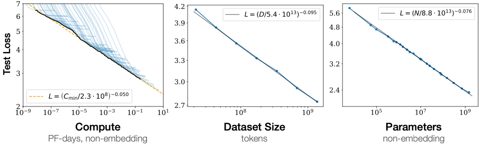
Research shows that increasing model size, dataset size, and compute used for training improves performance smoothly with no signs of saturation (Kaplan et al. 2020). Figure 4 demonstrates that test loss decreases predictably as each of these three factors increases, with no apparent ceiling in sight. Beyond training, AI-powered applications such as large-scale recommender systems and generative models require continuous inference at scale, consuming energy even after training completes. As AI adoption grows across industries from finance to healthcare to entertainment, the cumulative energy burden of AI workloads continues to rise, raising concerns about the environmental impact of widespread deployment.
Kaplan, J., S. McCandlish, T. Henighan, T. B. Brown, B. Chess, R. Child, S. Gray, A. Radford, J. Wu, and D. Amodei. 2020. “Scaling Laws for Neural Language Models.” ArXiv Preprint abs/2001.08361.
Beyond electricity consumption, the sustainability challenges of AI extend to hardware resource demands and the energy efficiency limitations of current architectures. Different processor types affect environmental impact through their energy characteristics. Using pJ/FLOP as a common comparison point, central processing units consume approximately 100 pJ/FLOP, graphics processing units achieve roughly 10 pJ/FLOP for dense tensor operations, specialized tensor processors reach about 1–2 pJ/FLOP, and fixed-function low-precision accelerators approach 0.1 pJ/operation.13 These hardware platforms require rare earth metals and complex manufacturing processes with embodied carbon.
13 pJ/FLOP and pJ/MAC: Energy-efficiency specifications often mix floating-point operations and multiply-accumulate operations. One MAC performs a multiply and an add, so direct comparisons require converting the unit convention and precision. The simplified hierarchy used here aligns with Table 2: CPUs at roughly 100 pJ/FLOP, GPUs around 10 pJ/FLOP for dense tensor operations, TPUs around 1–2 pJ/FLOP, and custom low-precision ASICs approaching 0.1 pJ/operation. This hierarchy defines the sustainability opportunity: choosing the right hardware tier for a given workload can reduce energy consumption by 100–1,000\(\times\) without any algorithmic changes.
The production of AI chips is energy-intensive, involving multiple fabrication steps that constitute a major portion of Scope 3 emissions in the overall AI system lifecycle. As model sizes continue to grow, the demand for AI hardware increases, exacerbating the environmental impact of semiconductor production and disposal.
Theoretical efficiency limits as a sustainability model
To understand the scale of AI’s energy challenge, it helps to compare current systems with the theoretical limits of computational efficiency. Modern large language models (LLMs) operate with an energy efficiency gap of \(10^6\times\) compared to the most efficient known physical implementations of pattern recognition and reasoning. This disparity establishes a “Sustainability Wall” where industrial-scale energy infrastructure is required to achieve tasks that theoretically require only milliwatts of power.
Training a single model like GPT-3 creates a stark reminder of this gap: while silicon-based systems consume megawatts to process \(10^{12}\) tokens, theoretical models of distributed processing suggest that similar cognitive capabilities are achievable with power budgets comparable to a household light bulb. This motivates the search for alternative computing paradigms that prioritize energy-aware architecture over raw throughput.
Principles of high-efficiency computing
Physical efficiency in information processing stems from three key principles that differ from current AI systems:
Selective, Event-Driven Activation: Rather than processing all information continuously, high-efficiency systems are asynchronous. They activate only small portions of the network at any time and consume energy only when actively processing changing signals.14
Local Learning and Sample Efficiency: Current architectures require training on trillions of tokens to achieve competence. High-efficiency models use strong inductive biases and self-supervised local learning to acquire capabilities from 10,000\(\times\) less data, reducing the cumulative energy cost of the training phase.
Sparsity and Sparse Interconnects: In modern GPUs, the majority of energy is spent on data movement and global synchronization. High-efficiency systems use sparse representations where only 1-2 percent of parameters are active for any given task, reducing bandwidth and switching energy by 50–100\(\times\).
14 Event-Driven Computing: A paradigm where computation triggers only on input changes rather than continuous clock cycles. Neuromorphic chips like Intel’s Loihi exploit this to achieve 100–1,000\(\times\) energy reductions for temporal tasks (audio, video, sensor data) by drawing near-zero power when inputs are static. The trade-off: event-driven architectures sacrifice throughput on batch workloads where all data changes simultaneously.
15 Spiking Neural Networks (SNNs): Third-generation neural networks that communicate through discrete spikes rather than continuous activations. SNNs process information only when spikes occur, achieving 10–100\(\times\) energy savings on temporal data (audio, video, sensor streams). The sustainability trade-off: current SNN training algorithms remain immature compared to backpropagation, limiting accuracy on standard benchmarks, but hardware implementations like Intel Loihi 2 demonstrate the efficiency ceiling these architectures can approach.
Prakash, Shvetank, Matthew Stewart, Colby Banbury, Mark Mazumder, Pete Warden, Brian Plancher, and Vijay Janapa Reddi. 2023. “Is TinyML Sustainable? Assessing the Environmental Impacts of Machine Learning on Microcontrollers.” ArXiv Preprint abs/2301.11899.
The biological model points toward promising research directions for sustainable AI. Architectures that implement Spiking Neural Networks (SNNs) or sparse activation patterns can achieve significant energy reductions by mimicking sparse communication models15 (Prakash et al. 2023). Local learning algorithms and self-supervised approaches offer additional pathways toward more sample-efficient and energy-conscious systems.
Achieving sustainable AI requires a systematic shift in system design, moving from continuously active, dense architectures toward event-driven, sparse computation models. As compute demands outpace incremental efficiency improvements in silicon manufacturing, addressing AI’s environmental impact demands rethinking the fundamental “Physics” of the algorithm based on these efficiency principles.
Figure 5 shows how six successive intervention steps combine to reduce the energy gap by approximately 10,000\(\times\), transforming an intractable divergence into an engineering challenge. No single lever is sufficient; closing the gap requires simultaneous progress across algorithmic, hardware, and systemic fronts.

The convergence of exponential computational demands with hard physical efficiency limits creates an unsustainable trajectory that threatens the long-term viability of AI scaling. To alter this trajectory, we must move beyond back-of-the-envelope calculations and establish rigorous, systemic frameworks for measuring and assessing energy consumption across the entire ML infrastructure.
Self-Check: Question
A hyperscaler commits to a 500 MW campus for a new training cluster, but the local grid interconnect approval is capped at 320 MW for the next three years. The company’s credit line would cover the projected electricity bill five times over. Which framing best captures why the chapter treats sustainability as a first-class engineering constraint rather than a reporting concern?
- Carbon accounting rules require disclosing the full planned capacity before any portion can be energized, so the 180 MW gap creates a compliance problem the team must file before training begins.
- Power-delivery and grid-interconnect capacity impose a physical ceiling that dollars cannot resolve on the required timescale, so the 180 MW gap becomes an infeasibility the training plan must route around.
- Electricity price volatility makes the 180 MW gap a budgeting risk, so the primary response is to hedge power contracts and continue the original training plan.
- Public concern about AI ethics will force the company to match every unapproved megawatt with offsets, adding cost but not changing what can be built.
A team plans a 10,000 MWh training run. Their procurement team can route it to Quebec at roughly 20 gCO2/kWh or Poland at roughly 800 gCO2/kWh, or invest six engineer-months in a 15 percent algorithmic speedup that runs at the Poland site. Using the section’s carbon-intensity reasoning, justify which lever the team should pull first and quantify the difference.
True or False: Because specialized accelerators have delivered order-of-magnitude energy-efficiency gains each hardware generation, a team can plan a decade-long AI strategy that relies on continued silicon improvements alone to keep total datacenter power flat.
Order the following events during a synchronized gradient-update step in a large training cluster when they create a grid-side transient: (1) GPUs resume a compute phase and cluster draw returns toward peak, (2) on-site batteries or supercapacitors absorb the dip and smooth the voltage, (3) thousands of GPUs simultaneously pause for AllReduce, causing a sudden drop in cluster power draw.
A research group wants to cut AI energy use without assuming the grid will keep scaling. Which architectural direction most directly attacks the root cause of the inefficiency the section identifies?
- Keeping every layer and attention head active on every input so utilization is always high, because higher utilization always means better efficiency.
- Event-driven and sparse-activation architectures that compute only on changes or salient inputs, because most of today’s energy pays for dense, globally synchronized data movement.
- Replacing all ReLU activations with a different pointwise nonlinearity to shave a small fraction of arithmetic per layer.
- Deferring sustainability work until emissions reporting standards stabilize, because architectural choices cannot be justified without fixed metrics.
Energy Measurement and Modeling
Engineers cannot optimize what they cannot measure. A cluster consuming five megawatts during a large language model training run directs only a fraction of that power into matrix multiplications; the remainder is consumed by cooling fans removing the resulting heat. Effective energy modeling requires decomposing the monolithic data center power bill into granular, component-level metrics that engineers can target for optimization.
The data center infrastructure foundations from Compute Infrastructure established power and cooling as dominant engineering constraints. Systematic measurement transforms these constraints into actionable sustainability metrics across three critical areas: energy consumption tracking during training and inference, carbon footprint analysis across system lifecycles, and resource usage assessment for hardware and infrastructure. Just as performance engineering requires profiling before optimization, sustainable AI engineering requires measurement before mitigation.
Carbon footprint analysis
Carbon footprint analysis provides the foundation for making informed design decisions about AI system sustainability. As AI systems continue to scale, systematic measurement of energy consumption and resource demands enables proactive approaches to environmental optimization. Developers and companies that build and deploy AI systems must consider not only performance and efficiency but also the environmental consequences of their design choices.
A central ethical challenge lies in balancing technological progress with ecological responsibility. The pursuit of increasingly large models often prioritizes accuracy and capability over energy efficiency, creating exponential increases in carbon emissions. While optimizing for sustainability may introduce trade-offs such as 10 to 30 percent longer development cycles or 1 to 5 percent accuracy reductions through techniques like pruning and quantization, these costs are substantially outweighed by environmental benefits. Integrating environmental considerations into AI system design has become an ethical imperative. The shift demands new industry norms: energy-aware training techniques, low-power hardware designs, and carbon-conscious deployment strategies (Patterson et al. 2021).
The ethical imperative extends beyond sustainability to encompass broader concerns related to transparency, fairness, and accountability. Figure 6 frames these concerns as connected environmental-justice and accountability trade-offs: transparency gaps obscure energy and carbon costs, fairness failures distribute harms unevenly, and weak accountability makes resource consumption difficult to trace. These concerns extend to sustainability, as the environmental trade-offs of AI development are often opaque and difficult to quantify. The lack of traceability in energy consumption and carbon emissions can lead to unjustified actions, where companies prioritize performance gains without fully understanding or disclosing the environmental costs.

Addressing these concerns demands greater transparency and accountability from AI companies. Large technology firms operate extensive cloud infrastructures that power modern AI applications, yet their environmental impact remains opaque. Organizations must measure, report, and reduce their carbon footprint throughout the AI lifecycle, from hardware manufacturing to model training and inference. Voluntary self-regulation provides an initial step, but policy interventions and industry-wide standards may be necessary to ensure long-term sustainability. Reported metrics such as energy consumption, carbon emissions, and efficiency benchmarks can hold organizations accountable.
Ethical AI development requires open discourse on environmental trade-offs. Researchers must advocate for sustainability within their institutions and organizations, ensuring that environmental concerns are integrated into AI development priorities. The broader AI community has begun addressing these issues, as exemplified by an open letter advocating a pause on large-scale AI experiments, which highlights concerns about unchecked expansion (Future of Life Institute 2023). Fostering a culture of transparency and ethical responsibility allows the AI industry to align technological advancement with ecological sustainability.
Future of Life Institute. 2023. Pause Giant AI Experiments: An Open Letter. Future of Life Institute open letter.
AI has the potential to reshape industries and societies, but its long-term viability depends on responsible development practices. Ethical AI development involves preventing harm to individuals and communities while ensuring that AI-driven innovation does not occur at the cost of environmental degradation. As stewards of these technologies, developers and organizations must integrate sustainability into AI’s future trajectory.
Preventing environmental harm requires us to hold AI systems accountable for their resource usage with the same rigor we apply to latency or accuracy. To achieve this transparency, we must translate abstract power consumption metrics into the universally recognized metric of environmental impact: the carbon footprint calculation.
Checkpoint 1.2: Lifecycle carbon estimation
Calculate the total carbon footprint for training a 70B parameter model.
Parameters: 2,048 H100 GPUs, 30 days, 700 W TDP, PUE 1.3, grid intensity 400 g \(\text{CO}_2\)/kWh.
Operational: Power = 2,048 \(\times\) 0.7 kW \(\times\) 1.3 \(\approx\) 1,864 kW. Energy = 1,864 kW \(\times\) 24h \(\times\) 30 \(\approx\) 1.34 million kWh. Emissions \(\approx\) 537 metric tons \(\text{CO}_2\).
Embodied: Assume manufacturing footprint is \(\approx\) 164 kg \(\text{CO}_2\) per H100 GPU (NVIDIA’s product carbon footprint). Amortized for 1 month of a 3-year cycle: (2,048 \(\times\) 164 kg) / 36 months \(\approx\) 9.3 metric tons.
Total: 537 + 9.3 \(\approx\) 546 metric tons \(\text{CO}_2\).
Translating power consumption into carbon emissions is only the first measurement challenge. A systematic lifecycle assessment across the full hardware lifecycle reveals where carbon emissions concentrate and where engineering interventions yield the greatest returns.
Three-phase lifecycle assessment framework
Effective carbon footprint measurement requires systematic analysis across three distinct phases that collectively determine environmental impact:
For training-centric research workloads, the training phase often dominates operational emissions because mathematical optimization requires sustained parallel computation16. As demonstrated by the GPT-3 case study, large language model training runs exemplify this energy intensity. Geographic placement affects emissions: moving an identical workload between hydro-heavy and coal-heavy grids can create tens-fold differences in carbon intensity.17
16 Optimizer Memory as Energy Cost: Adaptive Moment Estimation (Adam) requires 3\(\times\) the memory of plain SGD because it stores per-parameter first and second moment estimates alongside the weights themselves. For a 70B model in FP32, this means 840 GB of optimizer state. The sustainability implication is direct: larger optimizer state means more HBM accesses per training step, and at 100 pJ/byte for DRAM, memory overhead can dominate the energy budget of parameter updates.
17 Carbon Intensity Variance: Grid carbon intensity spans two orders of magnitude: coal at 820 g CO2/kWh vs. hydro at 10–30 g CO2/kWh. Critically, intensity also varies temporally: Texas fluctuates 10\(\times\) within a single day based on wind generation. This dual geographic and temporal variance is what makes carbon-aware scheduling viable: identical training runs can differ by 40–75\(\times\) in emissions based solely on when and where they execute.
For high-volume production services, the inference phase can dominate lifetime emissions because model serving repeats continuously after the training run is complete. While individual inferences require less computation than training, the cumulative impact scales with deployment breadth and usage frequency. Models serving millions of users generate ongoing emissions that can exceed training costs over extended deployment periods.
The manufacturing phase contributes embodied carbon from hardware production, including semiconductor fabrication, rare earth mining, and supply chain logistics.18 Its share is smaller for long-running workloads on carbon-intensive grids, but it can reach 30–50 percent of lifetime emissions on clean grids or low-utilization hardware. Often overlooked, this phase represents irreducible baseline emissions independent of operational efficiency.
18 Embodied Carbon: The CO2 emitted during manufacturing, transport, and disposal before a device computes its first FLOP. A single H100 embodies 150–200 kg CO2 from fabrication alone; at 700 W on the average U.S. grid, continuous operation matches embodied carbon in roughly three to four weeks. As data centers shift to renewables, embodied carbon’s share of total lifetime emissions grows, potentially exceeding 30 percent, making hardware refresh cycles a first-order sustainability decision.
Geographic and temporal optimization
Carbon intensity varies across geographic locations and time periods, creating optimization opportunities. Temporal scheduling can reduce emissions by 50–80 percent by aligning compute workloads with renewable energy availability, such as peak solar generation during daylight hours (Patterson et al. 2022). Carbon-aware scheduling systems can automatically shift nonurgent training jobs to regions and times with lower carbon intensity.
Patterson, David, Joseph Gonzalez, Quoc Le, Maud Texier, and Jeff Dean. 2022. “Carbon-Aware Computing for Sustainable AI.” Communications of the ACM 65 (11): 50–58.
Measuring carbon footprint during development requires integrating tracking tools into ML workflows. Listing 1 demonstrates how the CodeCarbon library wraps model training to capture real-time emissions data, enabling data-driven sustainability decisions.
from codecarbon import EmissionsTracker
import torch

# Initialize carbon tracking
tracker = EmissionsTracker()
tracker.start()

# Your model training code
model = torch.nn.Linear(100, 10)
optimizer = torch.optim.Adam(model.parameters())

for epoch in range(100):
    # Training step
    loss = model(data).mean()
    loss.backward()
    optimizer.step()

# Get emissions report
emissions = tracker.stop()
print(f"Training emissions: {emissions:.4f} kg CO2")
Integration of energy tracking into the development workflow allows engineers to make informed decisions about model complexity vs. environmental impact during development.
Power modeling fundamentals
Understanding where energy goes in AI systems requires grounding in the physics of digital computation. The CMOS power equation provides the foundation for reasoning about energy consumption in modern processors, explaining why different optimization techniques achieve their efficiency gains and enabling quantitative comparison of architectural choices.
The CMOS power equation
Every digital circuit consumes power through two fundamental mechanisms. Dynamic power arises from switching transistors between states, while static power results from leakage current that flows even when transistors are nominally off. Equation 1 formalizes the total power consumption:
\[P_{\text{total}} = P_{\text{dynamic}} + P_{\text{static}} = \alpha C V^2 f + V I_{\text{leak}} \tag{1}\]
The dynamic power component \(P_{\text{dynamic}} = \alpha C V^2 f\) depends on four parameters. The switching activity factor \(\alpha\) represents the fraction of transistors changing state per clock cycle, ranging from 0 to 1. General-purpose CPUs typically exhibit \(\alpha \approx 0.1\) to \(0.3\) due to diverse instruction mixes, while specialized AI accelerators can achieve \(\alpha \approx 0.6\) to \(0.8\) through optimized dataflow that keeps more circuits active during computation. The load capacitance \(C\) scales with transistor count and interconnect length. Supply voltage \(V\) enters quadratically, making voltage reduction the highest-impact lever for energy efficiency. Clock frequency \(f\) determines operations per second.
The static power component \(P_{\text{static}} = V \cdot I_{\text{leak}}\) represents leakage current that increases exponentially with temperature, approximately doubling for every 10 degrees Celsius rise. This thermal dependence creates a feedback loop: higher power generates heat, which increases leakage, which generates more heat. Managing this thermal runaway constrains the power density achievable in modern processors and explains why cooling infrastructure represents such a significant fraction of data center energy consumption (Dayarathna et al. 2016).
Dayarathna, Miyuru, Yonggang Wen, and Rui Fan. 2016. “Data Center Energy Consumption Modeling: A Survey.” IEEE Communications Surveys &Amp; Tutorials 18 (1): 732–94. https://doi.org/10.1109/comst.2015.2481183.
The practical implications for AI systems follow directly from these physics. The quadratic voltage dependence means that reducing voltage from 1.0V to 0.8V decreases dynamic power by 36 percent, even before considering that lower voltages often enable frequency reduction with additional linear savings. This relationship explains why specialized AI accelerators operating at lower voltages but higher utilization can achieve order-of-magnitude efficiency improvements over general-purpose processors.
Why optimization techniques save energy
The power equation illuminates why specific optimization techniques achieve their efficiency gains. Quantization reduces numerical precision from 32-bit floating point to 8-bit integers, which directly reduces datapath capacitance \(C\) by approximately 4 times since narrower datapaths require fewer transistors and shorter interconnects. Additionally, lower precision arithmetic enables reduced supply voltage \(V\) because the circuits have larger noise margins. The combined effect yields 6 to 10 times energy reduction per operation, closely matching published measurements of INT8 vs. FP32 inference efficiency.
Pruning removes weights from neural networks, reducing the effective capacitance \(C\) by eliminating computation paths that would otherwise consume switching energy. Structured pruning, which removes entire channels or attention heads, achieves larger efficiency gains than unstructured pruning because it eliminates complete circuit paths rather than individual operations that the hardware must still orchestrate.
Specialized accelerators improve the activity factor \(\alpha\) by designing circuits specifically for matrix multiplication and convolution operations. Where a CPU might activate 10 percent of its transistors during typical ML workloads, a systolic array architecture can keep 70 percent or more of its compute units active, effectively performing more useful work per watt of power consumed.
Facility-level power metrics
Beyond chip-level power, data center infrastructure imposes additional energy overhead. Equation 2 captures this relationship through the Power Usage Effectiveness (PUE) metric:
\[\text{PUE} = \frac{P_{\text{total\_facility}}}{P_{\text{IT\_equipment}}} \tag{2}\]
Napkin Math 1.4: PUE: The cost of cooling
Problem: A team operates a 2.0 MW cluster. If the facility can be optimized from the industry average PUE (1.58) to state-of-the-art (1.10), how much energy and money does that save annually?
Math: Energy saved is the difference in infrastructure overhead \((\text{PUE}-1)\) across the IT load.
- Overhead Reduction: 1.58 - 1.10 = 0.48.
- Annual energy savings: \(2.0 \text{ MW} \times 0.48 \times 8,760 \text{ hours} \approx\) 8,410 MWh.
- Financial Savings: 8,410 MWh \(\times\) $70/MWh \(\approx\) $588,672.
Systems insight: Infrastructure optimization is as valuable as algorithmic optimization. Dropping PUE by 0.48 is equivalent to discovering an algorithmic “free lunch” that makes the entire model 30 percent more efficient without changing a single line of training code. For large operators, cooling efficiency is the primary economic lever for sustainability.
A PUE of 1.0 would indicate perfect efficiency where all energy powers computation, though this is physically impossible since cooling, power distribution, and lighting require nonzero energy. Industry-average data centers operate at PUE of 1.5 to 2.0, meaning that 50 percent to 100 percent additional energy beyond computation goes to infrastructure (Davis et al. 2022). Leading hyperscale facilities achieve PUE between 1.1 and 1.2 through advanced cooling techniques including free-air cooling in cold climates, liquid cooling for high-density GPU clusters, and optimized power distribution.
Davis, Jacqueline, Daniel Bizo, Andy Lawrence, Owen Rogers, and Max Smolaks. 2022. Uptime Institute Global Data Center Survey 2022. Uptime Institute.
Equation 3 formalizes Water Usage Effectiveness (WUE), capturing the water consumption that evaporative cooling and other processes require:
\[\text{WUE} = \frac{W_{\text{annual\_water\_usage}}}{P_{\text{IT\_equipment\_energy}}} \tag{3}\]
The units are liters per kilowatt-hour, with typical values ranging from 0.5 to 2.0 L/kWh depending on climate and cooling technology. A data center with WUE of 1.8 L/kWh training a model requiring 10,000 MWh would consume 18 million liters of water, equivalent to roughly 40–50 US household-years of water use under a 380,000–450,000 L/year household baseline.
Facility-level metrics identify where engineering intervention yields the greatest returns. The following case study demonstrates how ML-driven optimization of PUE translates directly into measurable energy savings.
Case study: DeepMind energy efficiency
Google’s data centers form the backbone of services such as Search, Gmail, and YouTube, handling billions of queries daily (Centers 2023). These facilities require substantial electricity consumption, particularly for cooling infrastructure that ensures optimal server performance. Improving data center energy efficiency has long been a priority, but conventional engineering approaches faced diminishing returns due to cooling system complexity and highly dynamic environmental conditions (Buyya et al. 2010). To address these challenges, Google collaborated with DeepMind to develop a machine learning optimization system that automates and enhances energy management at scale.
Centers, Google Data. 2023. Efficiency: How We Do It.
Buyya, Rajkumar, Anton Beloglazov, and Jemal Abawajy. 2010. “Energy-Efficient Management of Data Center Resources for Cloud Computing: A Vision, Architectural Elements, and Open Challenges.” arXiv Preprint arXiv:1006.0308, ahead of print. https://doi.org/10.48550/arXiv.1006.0308.
After more than a decade of efforts to optimize data center design, energy-efficient hardware, and renewable energy integration, DeepMind’s AI approach targeted cooling systems, among the most energy-intensive aspects of data centers. Traditional cooling relies on manually set heuristics that account for server heat output, external weather conditions, and architectural constraints. These systems exhibit nonlinear interactions, so simple rule-based optimizations often fail to capture the full complexity of their operations. The result was suboptimal cooling efficiency, leading to unnecessary energy waste.
DeepMind’s team trained a neural network model using Google’s historical sensor data, which included real-time temperature readings, power consumption levels, cooling pump activity, and other operational parameters. Building on Jim Gao’s earlier work demonstrating that machine learning could predict data center PUE with 99.6 percent accuracy (Gao 2014), the model learned the intricate relationships between these factors and could dynamically predict the most efficient cooling configurations. Unlike traditional approaches that relied on human engineers periodically adjusting system settings, the AI model continuously adapted in real time to changing environmental and workload conditions.
Gao, J. 2014. Machine Learning Applications for Data Center Optimization. Google; Google White Paper.
19 PUE Optimization via ML: Google’s best facilities achieve PUE 1.08, meaning only 8 percent energy overhead for cooling and power distribution. DeepMind’s reinforcement-learning controller reduced cooling energy by 40 percent by exploiting nonlinear interactions between chillers, pumps, and ambient conditions that rule-based systems miss. This is a rare positive feedback loop where AI improves the efficiency of the infrastructure that powers AI.
Barroso, Luiz André, Urs Hölzle, and Parthasarathy Ranganathan. 2019. The Datacenter as a Computer: Designing Warehouse-Scale Machines. Synthesis Lectures on Computer Architecture. Springer International Publishing. https://doi.org/10.1007/978-3-031-01761-2.
Evans, Richard, and Jim Gao. 2016. DeepMind AI Reduces Google Data Centre Cooling Bill by 40%. DeepMind Blog.
The results demonstrated significant efficiency gains. When deployed in live data center environments, DeepMind’s AI-driven cooling system reduced cooling energy consumption by 40 percent, leading to an overall 15 percent improvement in PUE19 (Barroso et al. 2019; Evans and Gao 2016). For a facility operating at the industry-average PUE of 1.5 from Equation 2, a 15 percent improvement reclaims a substantial fraction of the energy lost to cooling overhead. These improvements were achieved without additional hardware modifications, demonstrating the potential of software-driven optimizations to reduce AI’s carbon footprint.
The DeepMind case study illustrates a rare positive feedback loop: machine learning optimizing the infrastructure that powers machine learning. The framework generalizes across facility designs and climate conditions, offering a scalable approach for global data center networks.
Carbon intensity and regional variation
The carbon impact of electricity consumption depends critically on the energy generation mix, quantified by carbon intensity measured in grams of CO2 equivalent per kilowatt-hour (g CO2eq/kWh). Table 1 quantifies how dramatically these intensities vary across energy sources:
| Energy Source | Carbon Intensity (g CO2eq/kWh) | Regional Examples |
|---|---|---|
| Coal | 820 to 1,200 | Poland, West Virginia |
| Natural Gas | 350 to 500 | Texas combined cycle plants |
| Solar PV | 20 to 50 | California, Arizona |
| Wind | 7 to 15 | Denmark, Scotland |
| Hydroelectric | 10 to 30 | Quebec, Norway |
| Nuclear | 5 to 20 | France, Ontario |
Geographic optimization can reduce carbon emissions by 10–50\(\times\) through strategic training location selection, as Figure 7 illustrates across representative regions.

Systematic energy metrics
Quantifying energy efficiency requires systematic metrics that enable comparison across hardware architectures and algorithmic approaches. These metrics provide the foundation for reasoning about optimization trade-offs and identifying bottlenecks in AI system energy consumption.
Energy per operation
The fundamental metric for computational energy efficiency is energy consumed per operation, typically measured in picojoules. For AI workloads, the most relevant metrics are energy per floating-point operation and energy per multiply-accumulate, where one MAC operation performs both a multiplication and addition, equivalent to two FLOPs.
Hardware architecture determines energy efficiency across orders of magnitude, spanning nearly four orders of magnitude from general-purpose CPUs to specialized analog accelerators. Table 2 quantifies these differences:
| Architecture | Energy Efficiency (pJ/FLOP or pJ/MAC) | Characteristics |
|---|---|---|
| CPU (general) | 100 pJ/FLOP | Low utilization, high flexibility |
| GPU (tensor cores) | 10 pJ/FLOP | High throughput, parallel execution |
| TPU (systolic array) | 1-2 pJ/FLOP | Specialized matrix operations, optimized dataflow |
| Google Edge TPU | 2-4 pJ/FLOP | On-device inference, INT8 optimized |
| ARM Ethos-U55 | 0.5-2 pJ/MAC | Microcontroller NPU, sub-watt TinyML |
| Maxim MAX78000 | 0.3-1 pJ/MAC | CNN accelerator with local weight storage |
| ASIC (INT8) | 0.1 pJ/operation | Fixed-function, low precision |
| Analog/In-Memory Compute | 0.01-0.1 pJ/MAC | Emerging technology, compute in memory array |
The four-order-of-magnitude spread reflects both circuit-level efficiency and architectural choices affecting utilization. CPUs execute diverse instruction mixes with low average utilization of arithmetic units. GPUs achieve higher utilization through massive parallelism. TPUs and ASICs maximize utilization through specialized datapaths optimized for specific operation types.
Precision directly affects energy per operation. INT8 integer arithmetic consumes approximately one-sixteenth the energy of FP32 floating-point at the same frequency and voltage. This combines reduced datapath capacitance of 4\(\times\) from bit width with lower voltage requirements of 2\(\times\) from larger noise margins and simpler control logic of 2\(\times\) from reduced complexity.
Energy per byte
Data movement often dominates energy consumption in modern AI systems. The energy cost of memory access spans five orders of magnitude across the storage hierarchy:
Table 3 reveals a critical insight: moving data from DRAM consumes 10 to 100 times more energy than performing arithmetic operations. For a GPU operating at 10 pJ/FLOP, accessing one FP32 operand from DRAM (4 bytes times 100 pJ/byte = 400 pJ) costs 40 times more than the computation itself. This energy gap drives architectural innovations including:
| Memory Level | Energy Cost (pJ/byte) | Access Latency |
|---|---|---|
| Register | 0.1 pJ/byte | 1 cycle |
| L1 Cache | 1 pJ/byte | 3-5 cycles |
| L2 Cache | 5 pJ/byte | 10-20 cycles |
| DRAM | 100 pJ/byte | 200-300 cycles |
| NVMe SSD | 1,000 pJ/byte | 50,000-100,000 cycles |
| Network | 10,000+ pJ/byte | Millions of cycles |
- On-chip memory for data reuse (NVIDIA tensor cores with shared memory)
- Optimized data layouts minimizing DRAM access (Google TPU systolic arrays)
- Compression reducing data movement (sparse tensor representations)
Arithmetic intensity and energy roofline
The balance between computation and data movement determines whether energy consumption is compute-bound or memory-bound. Equation 4 defines arithmetic intensity (AI), the ratio that determines which resource dominates energy consumption:
\[\text{AI} = \frac{\text{Total FLOPs}}{\text{Total Bytes Moved}} \tag{4}\]
Arithmetic intensity measured in FLOPs per byte determines the dominant energy consumer. Equation 5 expresses total energy as the sum of compute and memory contributions, while Equation 6 isolates the roofline-style dominant term:
\[E_{\text{total}} = E_{\text{compute}} + E_{\text{memory}} = \text{FLOPs} \times e_{\text{flop}} + \text{Bytes} \times e_{\text{byte}} \tag{5}\]
\[E_{\text{dominant}} = \max\left(E_{\text{compute}}, E_{\text{memory}}\right) = \max\left(\text{FLOPs} \times e_{\text{flop}}, \text{Bytes} \times e_{\text{byte}}\right) \tag{6}\]
where \(e_{\text{flop}}\) is energy per FLOP and \(e_{\text{byte}}\) is energy per byte moved. The maximum term identifies the dominant bottleneck for roofline reasoning; it is not the full energy in balanced cases. Equation 7 defines the crossover arithmetic intensity where compute and memory energy balance:
\[\text{AI}_{\text{crossover}} = \frac{e_{\text{byte}}}{e_{\text{flop}}} \tag{7}\]
For a GPU with \(e_{\text{flop}} = 10\) pJ/FLOP and \(e_{\text{byte}} = 100\) pJ/byte (DRAM access):
\[\text{AI}_{\text{crossover}} = \frac{100 \text{ pJ/byte}}{10 \text{ pJ/FLOP}} = 10 \text{ FLOPs/byte}\]
The energy roofline model (Figure 8) visualizes this relationship between arithmetic intensity and energy efficiency, revealing how different workload types are constrained by different bottlenecks.

To make this framework concrete, we can apply it to the most common operation in deep learning: matrix multiplication.
Example 1.1: MatMul energy analysis
Consider matrix multiplication \(C = A \times B\) for \(N{\times}N\) matrices in FP32 precision on a GPU with the energy characteristics above.
Step 1: Calculate FLOPs and bytes. - FLOPs: \(2N^3\) (one multiply-add for each of \(N^2\) output elements, accumulating over \(N\) elements) - Bytes: \(3N^2 \times 4\) bytes (read matrices \(A\) and \(B\), write matrix \(C\), each FP32 = 4 bytes) - Arithmetic intensity: \(\text{AI} = \frac{2N^3}{12N^2} = \frac{N}{6}\) FLOPs/byte
Step 2: Determine energy-limiting factor. For small matrices (\(N = 60\)):
- \(\text{AI} = 60/6 = 10\) FLOPs/byte (at crossover)
- Compute energy: \(2 \times 60^3 \times 10 \text{ pJ} = 4.32\,\mu\text{J} = 0.00432\) mJ
- Memory energy: \(3 \times 60^2 \times 4 \times 100 \text{ pJ} = 4.32\,\mu\text{J} = 0.00432\) mJ
- Balanced: both compute and memory contribute equally
For large matrices (\(N = 1000\)):
- \(\text{AI} = 1000/6 = 167\) FLOPs/byte (compute-bound)
- Compute energy: \(2 \times 10^9 \times 10 \text{ pJ} = 20\) mJ (dominates)
- Memory energy: \(3 \times 10^6 \times 4 \times 100 \text{ pJ} = 1.2\) mJ (negligible)
- Optimization priority: Focus on compute efficiency
For element-wise operations (\(N = 1000\), vector addition):
- FLOPs: \(N = 1000\) (one addition per element)
- Bytes: \(3N \times 4 = 12,000\) bytes (read two vectors, write one)
- \(\text{AI} = 1000/12000 = 0.083\) FLOPs/byte (memory-bound)
- Compute energy: \(1000 \times 10 \text{ pJ} = 0.00001\) mJ (negligible)
- Memory energy: \(12000 \times 100 \text{ pJ} = 0.0012\) mJ (dominates)
- Optimization priority: Reduce data movement through fusion
The energy roofline model reveals why different optimization strategies suit different workloads. Large dense matrix operations benefit from faster arithmetic units. Memory-bound operations like element-wise kernels benefit from data layout optimization, kernel fusion to reduce memory round-trips, and on-chip memory utilization. This framework guides architectural and algorithmic choices for sustainable AI system design.
Energy measurement techniques
Quantifying AI system energy consumption requires measurement at multiple levels of the hardware stack, from chip-level instrumentation to facility-wide monitoring. Each measurement approach offers different granularity, accuracy, and overhead trade-offs that practitioners must understand to select appropriate methods for their use case.
Hardware power counters
Modern processors include dedicated circuitry for power measurement that software can query through manufacturer-provided interfaces. These hardware counters measure actual power draw rather than estimating from activity, providing ground-truth energy consumption data at microsecond resolution.
Intel’s Running Average Power Limit (RAPL) interface exposes power measurements for CPU packages, DRAM, and integrated graphics through model-specific registers (MSRs). RAPL reports energy consumption in microjoules with updates every millisecond, enabling fine-grained attribution of energy to specific code regions. Listing 2 demonstrates how to read RAPL counters and calculate average power draw during a training loop:
import subprocess
import time

from mlsysim.core.constants import ureg


def read_rapl_energy():
    """Read current RAPL energy counters.

    Requires root or perf permissions.
    """
    result = subprocess.run(
        [
            "cat",
            "/sys/class/powercap/intel-rapl/intel-rapl:0/energy_uj",
        ],
        capture_output=True,
        text=True,
    )
    return int(result.stdout.strip())  # Returns microjoules


# Measure training energy
start_energy = read_rapl_energy()
start_time = time.time()

# Training loop
for epoch in range(num_epochs):
    train_one_epoch(model, dataloader, optimizer)

end_energy = read_rapl_energy()
end_time = time.time()

energy_joules = ((end_energy - start_energy) * ureg.microjoule).m_as(
    ureg.joule
)
avg_power_watts = energy_joules / (end_time - start_time)
print(
    f"Training energy: {energy_joules:.2f} J, Average power: {avg_power_watts:.2f} W"
)
RAPL measurements exclude discrete GPUs, which require separate monitoring through vendor-specific interfaces.
GPU power monitoring
NVIDIA GPUs expose power measurements through the NVIDIA Management Library (NVML), accessible via the nvidia-smi command-line tool or programmatic bindings. GPU power monitoring reports instantaneous power draw, which can vary significantly during computation due to dynamic voltage and frequency scaling. Listing 3 implements a measurement loop that samples power at regular intervals, computing average and peak power over the inference workload:
import pynvml
import torch
import time

from mlsysim.core.constants import milliwatt, watt

pynvml.nvmlInit()
handle = pynvml.nvmlDeviceGetHandleByIndex(0)  # First GPU


def measure_inference_power(model, input_data, num_iterations=100):
    """Measure average GPU power during inference."""
    power_readings = []

    model.eval()
    with torch.no_grad():
        for _ in range(num_iterations):
            # Run inference
            _ = model(input_data)
            torch.cuda.synchronize()

            # Sample power and convert mW → W via pint.
            power_mw = pynvml.nvmlDeviceGetPowerUsage(handle)
            power_readings.append((power_mw * milliwatt).m_as(watt))

    avg_power = sum(power_readings) / len(power_readings)
    return avg_power


avg_power = measure_inference_power(model, sample_input)
print(f"Average inference power: {avg_power:.1f} W")
For accurate energy measurement rather than instantaneous power sampling, integrate power readings over time or use NVIDIA’s energy counter when available on data center GPUs.
Edge and mobile device energy measurement
The measurement techniques described earlier apply to data center hardware with built-in power monitoring capabilities. Edge devices and microcontrollers present fundamentally different measurement challenges: they lack built-in power counters, operate at milliwatt rather than kilowatt scales, and require external instrumentation for accurate energy profiling. As TinyML deployments expand to billions of devices, understanding edge energy measurement becomes essential for comprehensive sustainability assessment.
Hardware power monitors for embedded systems
Microcontrollers and edge processors require external current and voltage measurement to quantify energy consumption. Several instrumentation approaches provide different trade-offs between accuracy, resolution, and cost:
The INA219 and INA226 I2C-based current sensors provide affordable measurement for development and validation, sampling at rates sufficient to capture inference-level energy consumption. For research requiring nanosecond-resolution measurements of individual operations, instruments like the Joulescope JS220 measure current from sub-microamp sleep states through ampere-level active peaks, enabling characterization of the full dynamic range of edge AI workloads.
Mobile platform energy profiling
Mobile devices provide platform-specific APIs for energy attribution, though with less granularity than hardware monitors:
- Android PowerStats HAL: Provides per-component power attribution for CPU, GPU, NPU, and radio subsystems, enabling developers to identify which model operations dominate energy consumption.
- Qualcomm Trepn Profiler: Offers millisecond-resolution power measurement on Snapdragon platforms, correlating power traces with code execution for NPU workload optimization.
- ARM Streamline: Provides energy-annotated profiling for Cortex-A and Mali GPU platforms, enabling identification of inefficient kernel implementations.
- Apple Instruments Energy Log: Reports thermal state and energy impact scores for iOS applications, though without direct wattage measurements.
Mobile profiling tools integrate with development workflows, enabling iterative optimization of on-device inference energy consumption during model deployment. Table 4 summarizes the available instrumentation options across platforms, including resolution, accuracy, and integration requirements.
| Instrument | Resolution | Accuracy | Use Case |
|---|---|---|---|
| INA219/INA226 | 100 microsecond sampling | plus or minus 1 percent | Low-cost embedded profiling |
| PAC1934 | 1 millisecond, 4 channels | plus or minus 2 percent | Multi-rail MCU measurement |
| Joulescope JS220 | Sub-microsecond, nanoamp range | plus or minus 0.1 percent | Professional TinyML benchmarking |
| Otii Arc Pro | 10 microsecond, automation | plus or minus 0.5 percent | Automated battery life testing |
Edge measurement methodology
Edge energy measurement requires careful methodology to produce reproducible results:
Baseline characterization: Measure idle power consumption across all sleep states, as baseline power can vary from 1 microamp in deep sleep to 1 milliamp in idle active states on typical microcontrollers.
Warm-up Period: Execute 100 or more inference iterations before measurement to reach thermal equilibrium, as initial iterations may exhibit different power characteristics due to cache warming and voltage regulator settling.
Duty Cycle Accounting: Edge devices typically operate with significant idle periods between inferences. Report both peak inference power and average power at realistic duty cycles. Equation 8 expresses this relationship:
\[P_{\text{average}} = P_{\text{active}} \times D + P_{\text{idle}} \times (1 - D) \tag{8}\]
where \(D\) is the duty cycle (fraction of time performing inference).
- Peripheral Isolation: Disable or account for peripheral power consumption (sensors, radios, displays) when measuring model inference energy, as these can dominate total system power.
System-level energy profiling
Comprehensive energy accounting requires combining chip-level measurements with infrastructure overhead. Equation 9 formalizes total energy as the sum of component contributions scaled by facility overhead:
\[E_{\text{total}} = (E_{\text{CPU}} + E_{\text{GPU}} + E_{\text{memory}} + E_{\text{network}}) \times \text{PUE} \tag{9}\]
System-level profilers like Intel VTune, NVIDIA Nsight Systems, and open-source tools such as PowerJoular aggregate measurements across components. For production deployments, smart power distribution units (PDUs) at the rack level provide facility-verified measurements that include cooling overhead.
Equation 10 expresses the relationship between measured component power and total facility energy:
\[P_{\text{facility}} = P_{\text{IT}} \times \text{PUE} = (P_{\text{servers}} + P_{\text{network}} + P_{\text{storage}}) \times \text{PUE} \tag{10}\]
For a cluster consuming 1 MW of IT power in a facility with PUE of 1.4, total facility power consumption reaches 1.4 MW, with the additional 400 kW powering cooling, power conversion, and infrastructure systems.
Understanding that a PUE of 1.4 means an automatic 40 percent overhead on all computational power highlights the critical role of facility efficiency. However, operational power consumption is only one piece of the equation; to capture the true environmental cost of our systems, we must formalize how we convert raw kilowatts into tons of carbon emissions.
Self-Check: Question
A profiling run on an accelerator with approximately 10 pJ per FLOP of compute energy and approximately 100 pJ per byte of DRAM energy reports an arithmetic intensity of 3 FLOPs per byte for an attention kernel. Which optimization family is most likely to move this workload closer to the energy roofline?
- Replacing the accelerator with one that advertises 2x the peak FLOPS per watt while keeping the memory subsystem unchanged, because raising the compute ceiling always lowers energy.
- Fusing operators and tiling to keep intermediate activations in on-chip SRAM, because the kernel sits far to the left of the energy crossover at about 10 FLOPs per byte and pays most of its joules in DRAM traffic.
- Prioritizing a PUE reduction on the facility because chip-level bottlenecks do not affect per-query energy.
- Raising numerical precision from FP16 to FP32, because higher precision does more useful work per byte read.
A 2 MW cluster drops its PUE from 1.58 to 1.10 without changing any model code or hardware SKU. Explain why the chapter counts this as a first-order sustainability intervention, and quantify roughly what the facility saves per year.
An engineer must profile energy for a battery-powered microcontroller running a wake-word detector that sleeps most of the second. The device has no internal power counters and draws microwatts during deep sleep. Which measurement approach best matches the section’s edge methodology?
- Sample a tool such as nvidia-smi at 10 Hz and integrate the series, because server-grade sampling tools work across platforms.
- Use an external current-sense monitor such as an INA219 or Joulescope, sample at a rate that resolves the active burst and deep-sleep transitions, and explicitly account for duty cycle, warm-up, and peripherals.
- Estimate total energy by multiplying parameter count by a fixed J-per-parameter constant, because compute energy is the dominant term in TinyML.
- Rely on CPU-package RAPL counters, because they generalize from server CPUs to microcontroller-class devices.
A facility reports 4.2 MW of compute IT load and 6.3 MW of total site draw over the same hour. The sustainability team wants a single scalar that captures how much the non-IT infrastructure contributes to the total, so they can compare the site to peers year over year. Which metric gives them exactly that ratio, and what does a drop in it imply?
- Grid carbon intensity; a drop means the grid has decarbonized.
- Arithmetic intensity; a drop means the workload has become more memory-bound.
- PUE, computed as 6.3 / 4.2 = 1.5; a drop means every joule of useful IT work now carries less cooling and power-distribution overhead.
- Model FLOPs utilization; a drop means the accelerators are underused.
A profiling sweep across a training workload shows element-wise normalization and activation kernels spending roughly 8x more joules on HBM reads than on arithmetic. The service owner proposes four follow-ups. Which best matches the energy model this section develops?
- Upgrading to a newer accelerator with 2x peak tensor-core FLOPS, because more FLOPS always lowers total energy per step.
- Fusing the normalization and activation into adjacent matrix-multiply kernels so intermediate tensors stay in on-chip SRAM and round-trips to HBM collapse.
- Ignoring the kernel and investing only in carbon-aware scheduling, because chip-level energy is negligible once the grid is considered.
- Raising numerical precision to FP32 to make each byte of DRAM carry more useful arithmetic.
A team proposes to report total AI system energy as the simple sum of CPU, GPU, memory, and network component measurements. Explain why the section rejects this accounting and what form the corrected total must take.
Carbon Footprint Calculation
Consider a data center running on 100 percent renewable hydroelectric power. Its operational carbon emissions are effectively zero, but AI trained there is not carbon-free. Mining the silicon, manufacturing the GPUs, and pouring the concrete for the data center released thousands of tons of CO2 before the servers were ever turned on. A true carbon footprint calculation must account for both the energy consumed during operation and the “embodied carbon” emitted during construction.
Operational carbon calculation
Operational carbon emissions result from electricity consumption during training and inference, scaled by grid carbon intensity. Equation 11 quantifies this as the product of energy, grid carbon intensity, and facility overhead:
\[C_{\text{operational}} = E_{\text{total}} \times \text{CI}_{\text{grid}} \tag{11}\]
where \(E_{\text{total}}\) is the facility-level energy from Equation 9 (component energy already scaled by \(\text{PUE}\)) and \(\text{CI}_{\text{grid}}\) is the carbon intensity of the electricity grid. The facility overhead enters once, through \(E_{\text{total}}\), so it does not appear again in the carbon equation. A concrete training emissions calculation illustrates this framework.
Example 1.2: Training emissions calculation
Consider training a 7 billion parameter model on 64 A100 GPUs for 14 days:
Step 1: Compute energy. - GPU power: 400 W per A100 at typical training utilization - Training time: 14 days times 24 hours = 336 hours - GPU energy: 64 GPUs times 400 W times 336h = 8,601,600 Wh = 8,602 kWh
Step 2: Apply PUE. - Facility PUE: 1.2 (efficient hyperscale data center) - Total facility energy: 8,602 kWh times 1.2 = 10,322 kWh
Step 3: Calculate emissions. - Grid carbon intensity: 429 g CO2/kWh (US average) - Operational emissions: 10,322 kWh times 429 g/kWh = 4,428 kg CO2 = 4.4 metric tons
Comparison: Same training in low-carbon region
- Quebec grid intensity: 20 g CO2/kWh
- Emissions: 10,322 kWh times 20 g/kWh = 206 kg CO2
The geographic choice alone produces a 21-fold difference in training emissions.
Embodied carbon assessment
As Figure 9 illustrates, operational energy dominates total cost of ownership for typical deployments, but embodied carbon from semiconductor fabrication becomes the binding constraint as the grid shifts to renewables.

The key insight from Figure 9 is the shifting bottleneck: as grids decarbonize, embodied carbon from chip fabrication and data center construction becomes the dominant term, making hardware utilization and longevity the highest-leverage sustainability levers.
Embodied carbon encompasses emissions from raw material extraction, semiconductor fabrication, assembly, transportation, and end-of-life disposal. For AI hardware, manufacturing emissions are dominated by the energy-intensive nature of advanced semiconductor processes.
Advanced-node AI accelerators carry substantial manufacturing footprints: an NVIDIA A100 GPU embodies approximately 150 kg CO2eq per unit (Luccioni et al. 2023), and an H100 GPU embodies approximately 150 to 200 kg CO2eq (per NVIDIA’s product carbon footprint), including wafer fabrication at advanced process nodes, high-bandwidth memory production, and packaging. Equation 12 amortizes this embodied carbon over the hardware lifetime to compute per-use emissions:
\[C_{\text{embodied,daily}} = \frac{C_{\text{manufacturing}}}{T_{\text{lifetime}} \times 365} \tag{12}\]
Understanding how embodied carbon accumulates over time reveals why hardware utilization and lifetime dominate total lifecycle emissions.
Systems Perspective 1.2: Embodied carbon amortization
A hidden cost emerges when renting a GPU for an hour: the fee does not cover electricity alone but also amortizes the carbon debt of manufacturing.
Formula: \[C_{\text{total}} = C_{\text{operational}} + \left( \frac{C_{\text{manufacturing}}}{T_{\text{lifetime,years}} \times 365 \times 24} \times T_{\text{job,hours}} \right)\]
Scenario: Training a model for 10 hours on 8 NVIDIA H100s.
- Operational: 8 GPUs\(\times\) 0.7 kW\(\times\) 10h = 56 kWh. At 0.4 kg/kWh (gas grid) = 22.4 kg CO2.
- Embodied: 8 GPUs\(\times\) 164 kg/GPU = 1312 kg total.
- Amortization: Lifetime = 3 years (26,280 hours).
- Hourly “Rent” = \(1312/26280 \approx 0.050\) kg/hour.
- Job Cost = \(0.050 \times 10 =\) 0.50 kg CO2.
Systems insight: For long-lived hardware in dirty grids, electricity dominates (22.4 vs. 0.50). However, in clean grids (hydro, 0.02 kg/kWh), operational drops to 1.1 kg, making embodied carbon a significant fraction (~31 percent) of the total footprint.
For an accelerator with 164 kg embodied carbon (per NVIDIA’s product carbon footprint) and a 4-year data center lifetime:
The daily amortized embodied carbon is 164 kg / (4 \(\times\) 365) \(\approx\) 0.112 kg/day.
Over a 14-day training run using 64 accelerators:
The job’s amortized embodied carbon is 64 \(\times\) 14 \(\times\) 0.112 \(\approx\) 101 kg CO2.
The embodied contribution of 101 kg represents approximately 2.3 percent of the operational emissions (4,428 kg) calculated above for the US average grid. If training occurred in Quebec’s low-carbon grid, where the same run produced 206 kg of operational emissions, the embodied contribution would be about 33 percent of total emissions.
Lifecycle carbon accounting
Complete lifecycle assessment combines operational and embodied emissions across all phases. Equation 13 aggregates these contributions:
\[C_{\text{lifecycle}} = C_{\text{training}} + C_{\text{inference}} + C_{\text{embodied}} \tag{13}\]
As Figure 10 shows, training dominates this single-deployment lifecycle snapshot, while manufacturing and inference remain significant factors.

The carbon-lifecycle breakdown in Figure 10 shows training dominating a single-deployment snapshot, with manufacturing and inference taking smaller shares. The cumulative picture, however, is the opposite: a model serving millions of queries per day can exceed its entire training carbon footprint within months, or within days for higher-traffic services, making inference optimization the highest-impact sustainability intervention for production systems over a model’s service life.
For models deployed at scale, inference emissions often dominate the lifecycle. Consider a model serving 10 million queries per day at 0.001 kWh per query. The annual inference energy and emissions break down as follows:
- Daily energy: 10 million times 0.001 kWh = 10,000 kWh
- Annual energy: 10,000 times 365 = 3,650,000 kWh
- Annual emissions (US grid): 3,650,000 times 0.429 = 1,565,850 kg = 1,566 metric tons CO2
Compared with the 7B/64-A100 training example above (4.4 metric tons), cumulative inference emissions exceed training emissions after about 1.0 days of deployment at this scale. For frontier-scale training runs, the crossover can shift to weeks or months depending on query volume, per-query energy, and grid intensity.
The lifecycle perspective reveals a clear priority: optimize inference efficiency for widely-deployed models, and focus training efficiency efforts on models that undergo frequent retraining or experimental iteration.
Regional grid intensity data sources
Accurate carbon accounting requires reliable grid intensity data. Real-time carbon intensity varies with generation mix, which changes hourly based on demand, renewable availability, and plant dispatch decisions. Several data sources provide this information:
The US Energy Information Administration (EIA) publishes historical grid emissions factors by region, updated annually. For prospective analysis, these annual averages provide reasonable estimates. ElectricityMap and WattTime provide real-time carbon intensity APIs covering major grids worldwide, enabling carbon-aware scheduling systems. For retrospective analysis of completed training runs, hourly marginal emissions data from these sources enables accurate attribution. Listing 4 implements a lifecycle carbon calculator that integrates energy measurements with grid intensity data:
from mlsysim.core.constants import THOUSAND, hour, ureg, watt


def calculate_carbon_footprint(
    gpu_power_watts: float,
    num_gpus: int,
    training_hours: float,
    pue: float,
    grid_intensity_gco2_kwh: float,
    gpu_embodied_kg: float,
    gpu_lifetime_years: float,
) -> dict:
    """Calculate lifecycle carbon footprint for a training run."""

    # Operational emissions
    energy_wh = gpu_power_watts * num_gpus * training_hours
    energy_kwh = (energy_wh * watt * hour).m_as(ureg.kilowatt_hour)
    facility_energy_kwh = energy_kwh * pue
    # g CO2 → kg (mlsysim does not export mass pint units yet).
    operational_kg = (
        facility_energy_kwh * grid_intensity_gco2_kwh / THOUSAND
    )

    # Embodied emissions (amortized)
    daily_embodied = gpu_embodied_kg / (gpu_lifetime_years * 365)
    training_days = training_hours / 24
    embodied_kg = num_gpus * training_days * daily_embodied

    return {
        "energy_kwh": facility_energy_kwh,
        "operational_carbon_kg": operational_kg,
        "embodied_carbon_kg": embodied_kg,
        "total_carbon_kg": operational_kg + embodied_kg,
        "embodied_fraction": embodied_kg
        / (operational_kg + embodied_kg),
    }


# Example: 7B model training
result = calculate_carbon_footprint(
    gpu_power_watts=400,
    num_gpus=64,
    training_hours=336,  # 14 days
    pue=1.2,
    grid_intensity_gco2_kwh=429,  # US average
    gpu_embodied_kg=164,
    gpu_lifetime_years=4,
)
print(
    f"Total carbon footprint: {result['total_carbon_kg']:.0f} kg CO2"
)
print(f"Embodied fraction: {result['embodied_fraction']:.1%}")
Teams can integrate total lifecycle carbon accounting directly into their orchestration dashboards using this programmatic approach. Calculating operational and embodied emissions for individual training runs, however, captures only one dimension of the problem. The macro-level patterns of how modern AI data centers consume resources at scale reveal additional constraints and optimization opportunities.
Self-Check: Question
Two engineers disagree about how to report the carbon footprint of a training run that used leased GPUs in a hydro-powered region. Which framing correctly separates operational and embodied carbon per this section’s equations?
- Operational carbon is the manufacturing and shipping footprint of the GPUs, while embodied carbon is the grid electricity used while training.
- Operational carbon is the electricity used during training and inference multiplied by grid intensity and facility PUE, while embodied carbon is the pre-use footprint of hardware and construction amortized over useful lifetime.
- Operational carbon applies only to cloud training, while embodied carbon applies only to on-premises hardware.
- Operational carbon is a concern only on fossil-heavy grids, while embodied carbon is a concern only for edge devices.
A team moves a training run from a fossil-heavy grid at roughly 800 gCO2/kWh to a hydro-powered grid at roughly 20 gCO2/kWh. They are surprised when their sustainability dashboard shows embodied carbon becoming the dominant term rather than operational. Explain the mechanism that causes this inversion and what it implies for hardware decisions.
True or False: A model trained in a datacenter powered 100 percent by hydroelectricity can honestly be reported as having a zero carbon footprint for its training run.
A deployed model serves 10 million queries per day at 0.001 kWh per query. Its single training run consumed 1,287 MWh. Using the section’s lifecycle reasoning, what is the most important accounting consequence?
- Training still dominates because a training run uses specialized accelerators at higher per-chip peak power than serving.
- Embodied carbon can be ignored because inference energy is metered daily.
- Cumulative serving energy can exceed the one-time training energy within months — 10 million queries at 0.001 kWh is 10 MWh per day, so the 1,287 MWh training is matched in roughly 130 days — making inference efficiency the highest-impact production lever.
- The main optimization target should be compressing training time even if it raises per-query inference energy.
Order the following steps of a lifecycle carbon estimate for a training run: (1) amortize hardware manufacturing and construction emissions over device lifetime to compute the run’s embodied share, (2) compute total facility energy from IT energy and PUE, (3) aggregate operational and embodied components into the lifecycle total, (4) convert operational energy to operational carbon by multiplying by grid carbon intensity.
Data Center Energy and Resource Consumption
When a traditional web server handles an HTTP request, the CPU briefly spikes to 20 percent utilization and immediately returns to idle. When a GPU cluster trains a foundation model, thousands of processors run at 100 percent utilization, drawing maximum power continuously for three straight months. This unprecedented, unyielding thermal density fundamentally breaks traditional data center design, forcing engineers to adopt liquid cooling and redesign entire power distribution networks.
Data center energy and AI workloads
Data centers are the primary energy consumers for AI systems, and the variation in their power demands reveals both the scale of the challenge and specific optimization opportunities.
Data center energy efficiency varies significantly across facilities. Power Usage Effectiveness ranges from 1.1 in Google’s most efficient facilities to 2.5 in typical enterprise data centers, effectively doubling energy consumption through infrastructure overhead. Geographic location also impacts carbon intensity: the same model trained on a hydro-heavy grid can have tens-fold lower operational emissions than one trained on a coal-heavy grid under the representative intensities used earlier. Without access to renewable energy, these facilities rely heavily on nonrenewable sources such as coal and natural gas, contributing to global carbon emissions. IEA estimates data-center electricity-use emissions at about 180 Mt today, rising to around 300 Mt by 2035 in its Base Case while remaining below 1.5 percent of total energy-sector emissions.20 The energy burden of AI is expected to grow due to increasing data center capacity, rising AI training workloads, and increasing inference demands (Patterson et al. 2021). Without intervention, these trends risk making AI’s environmental footprint unsustainably large (Thompson et al. 2023; Dodge et al. 2022).
20 Data Center Emissions Scale: Data centers consume roughly 1–2 percent of global electricity today, with AI accelerating demand growth. IEA estimates emissions from data-center electricity use at about 180 Mt today, rising to around 300 Mt by 2035 in its Base Case and remaining below 1.5 percent of total energy-sector emissions. The largest hyperscale facilities draw over 100 MW continuously, equivalent to powering tens of thousands of homes, and AI workloads are the fastest-growing segment of that demand.
Thompson, Neil, Tobias Spanuth, and Hyrum Anderson Matthews. 2023. “The Computational Limits of Deep Learning and the Future of AI.” Communications of the ACM 66 (3): 48–57.
Dodge, Jesse, Taylor Prewitt, Remi Tachet des Combes, Erika Odmark, Roy Schwartz, Emma Strubell, Alexandra Sasha Luccioni, Noah A. Smith, Nicole DeCario, and Will Buchanan. 2022. “Measuring the Carbon Intensity of AI in Cloud Instances.” 2022 ACM Conference on Fairness Accountability and Transparency, 1877–94. https://doi.org/10.1145/3531146.3533234.
Energy demands in data centers
AI workloads are among the most compute-intensive operations in modern data centers. Companies such as Meta operate hyperscale data centers spanning multiple football fields in size, housing large fleets of AI-optimized servers.21 Unofficial estimates have suggested GPT-4 may have used on the order of tens of thousands of A100-class GPUs for months (SemiAnalysis 2023), but OpenAI has not disclosed GPT-4’s hardware, training compute, model size, or training duration. These facilities rely on high-performance AI accelerators like NVIDIA DGX H100 units, each of which can draw up to 10.2 kW at peak power (Choquette 2023). The energy efficiency gap becomes clear when comparing hardware generations. H100 GPUs achieve approximately 2.5 to 3\(\times\) better performance per watt than A100s for AI training workloads, while mixed-precision training can reduce energy consumption by 15 to 30 percent depending on model architecture and hardware through reduced computational precision with minimal accuracy impact (Gholami et al. 2021).
21 Hyperscale Data Center Footprint: Meta’s Prineville facility spans 230,000 m² and houses over 150,000 servers; major cloud fleets consume country-scale electricity annually. These physical scales matter for sustainability because each facility’s power demand (100–300 MW) locks in decades of grid-dependency decisions that no algorithmic optimization can undo.
SemiAnalysis. 2023. GPT-4 Architecture, Infrastructure, Training Dataset, Costs, Vision, MoE. SemiAnalysis Blog.
Choquette, J. 2023. “NVIDIA Hopper H100 GPU: Scaling Performance.” IEEE Micro 43 (3): 9–17. https://doi.org/10.1109/mm.2023.3256796.
Gholami, A., S. Kim, Z. Dong, Z. Yao, M. W. Mahoney, and K. Keutzer. 2021. “A Survey of Quantization Methods for Efficient Neural Network Inference.” arXiv Preprint arXiv:2103.13630, 291–326. https://doi.org/10.1201/9781003162810-13.
AI’s rapid adoption across industries drives this dramatic energy consumption. Figure 11 projects that AI workload energy demand will increase total data center energy use after 2024, with the AI segment growing from roughly 10 percent to about a quarter of total data center energy demand by 2030 (Masanet et al. 2020). Efficiency gains have historically offset rising power needs, but those gains are decelerating, amplifying AI’s environmental impact.
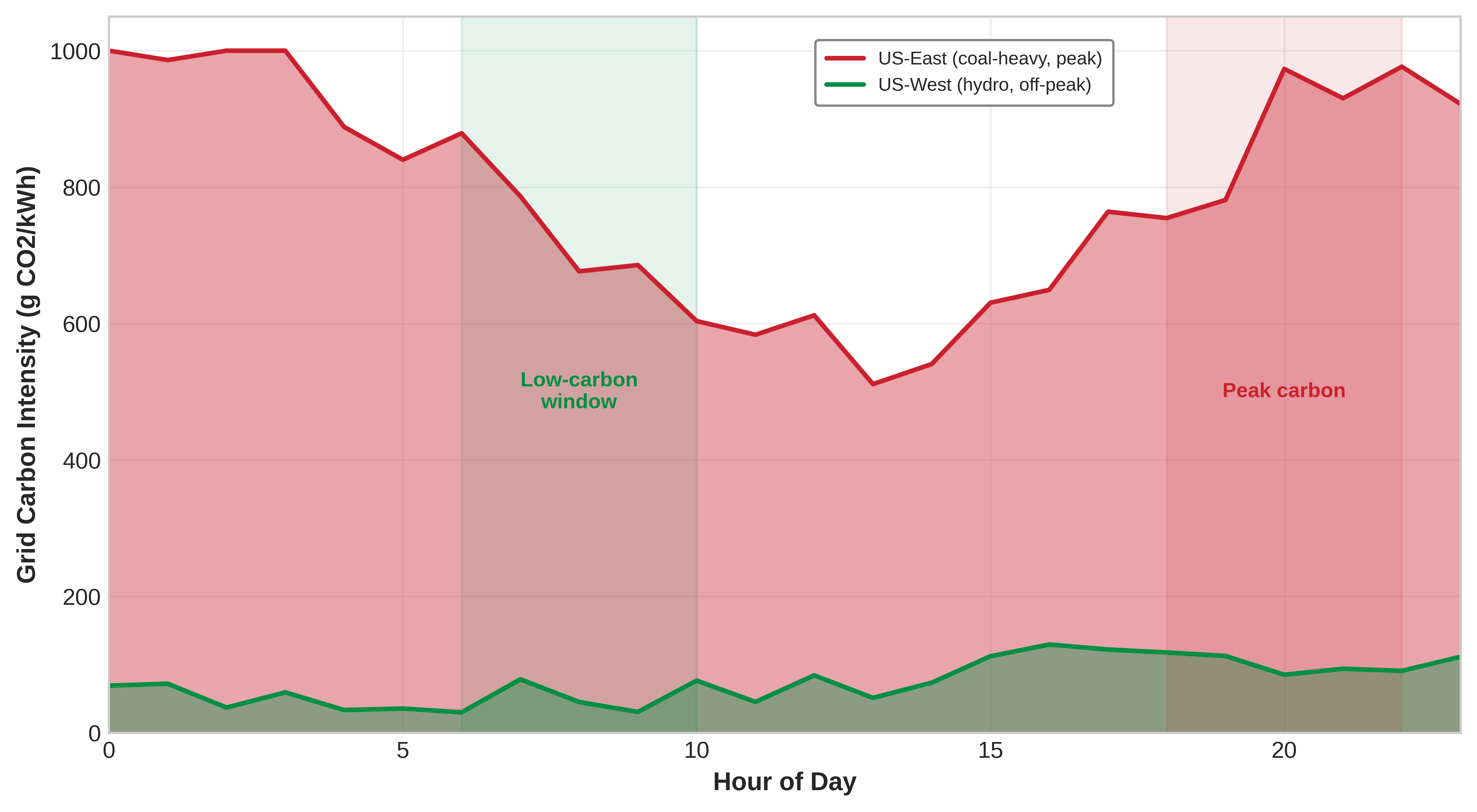
Masanet, Eric, Arman Shehabi, Nuoa Lei, Sarah Smith, and Jonathan Koomey. 2020. “Recalibrating Global Data Center Energy-Use Estimates.” Science 367 (6481): 984–86. https://doi.org/10.1126/science.aba3758.
Beyond computational demands, cooling accounts for 30–40 percent of data center energy consumption (Ebrahimi et al. 2014), as discussed in Section 1.7.3.
Ebrahimi, K., G. F. Jones, and A. S. Fleischer. 2014. “A Review of Data Center Cooling Technology, Operating Conditions and the Corresponding Low-Grade Waste Heat Recovery Opportunities.” Renewable Sustainable Energy Rev. 31: 622–38. https://doi.org/10.1016/j.rser.2013.12.007.
While Figure 11 projects global trends, the United States alone illustrates just how rapidly cloud and AI infrastructure are reshaping national energy planning. Figure 12 presents US data center electricity consumption data from the Lawrence Berkeley National Laboratory (LBNL), showing that consumption tripled from 58 TWh in 2014 to 176 TWh in 2023, with AI workloads becoming an increasingly important driver. LBNL projects a further doubling or tripling by 2028, with the high-end scenario implying that data centers would consume approximately 12 percent of US electricity. This trajectory represents a physical constraint on AI scaling that no software optimization alone can overcome.
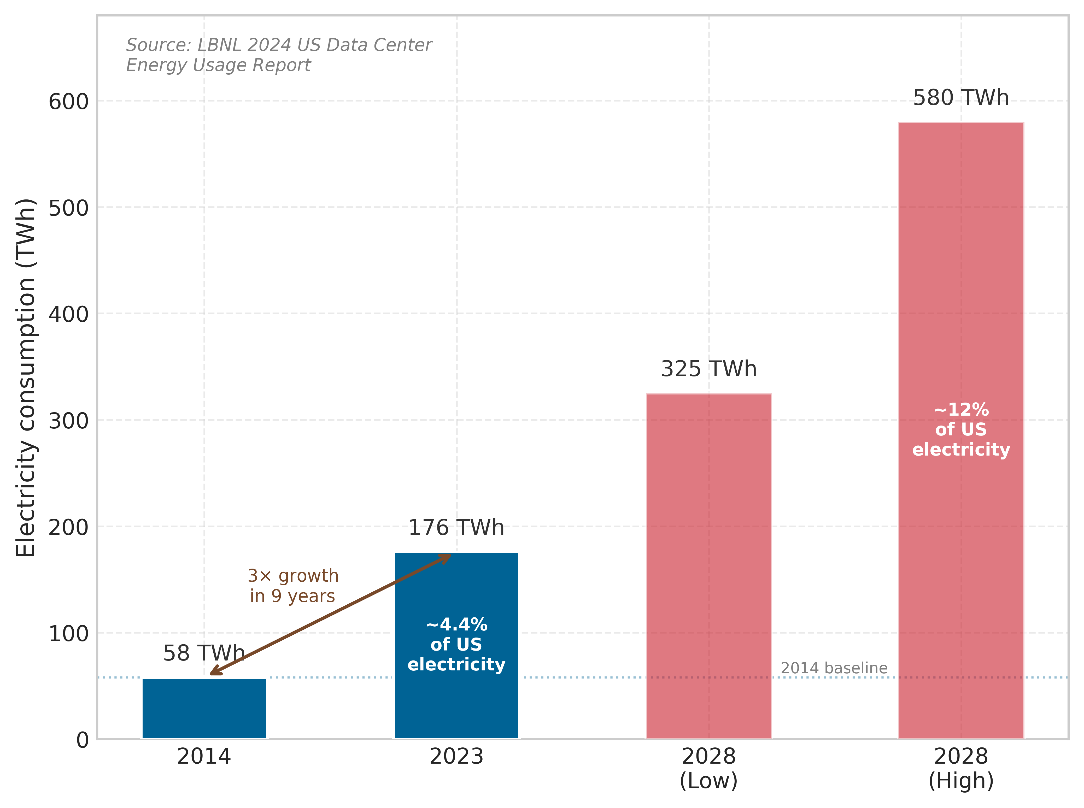
Distributed systems energy optimization
Large-scale AI training inherently requires distributed systems coordination, creating additional energy overhead that compounds computational demands. The parallelism strategies examined in Distributed Training Systems introduce network communication costs that can account for 20–40 percent of total energy consumption in large clusters.22 This coordination across thousands of GPUs requires constant synchronization of computational updates and model parameters23, generating data movement between nodes. This communication overhead scales poorly: increasing cluster size can increase networking energy superlinearly for all-to-all communication patterns in gradient aggregation.
22 Parallelism Energy Overhead: Data, model, and pipeline parallelism each impose distinct communication patterns with different energy costs. Data parallelism broadcasts gradients (bandwidth-bound); model parallelism exchanges activations every layer (latency-bound); pipeline parallelism introduces bubble overhead (utilization-bound). GPT-3 combined all three, and the choice of parallelism strategy can swing total training energy by 20–40 percent for the same model.
23 Gradient Synchronization Energy Cost: Ring-allreduce scales communication linearly with message size but requires every node to participate, meaning one slow node wastes energy across the entire ring. At scale, gradient compression (1-2 bit quantization) can reduce network energy by 10–50\(\times\) per synchronization step, but introduces statistical noise that may require additional training iterations, partially offsetting the savings.
Addressing these communication overheads, cluster-wide energy optimization requires coordinated resource management that extends beyond individual server efficiency. Dynamic workload placement can achieve 15–25 percent energy savings by consolidating training jobs onto fewer nodes during low-demand periods, allowing unused hardware to enter low-power states. Similarly, intelligent scheduling that coordinates training across multiple data centers can use time-zone differences and regional renewable energy availability, reducing carbon intensity by 30–50 percent through temporal load balancing.
Infrastructure sharing presents efficiency opportunities often overlooked in sustainability analyses. Multi-tenant training environments, where multiple model training jobs share the same cluster, can improve GPU utilization from typical 40–60 percent to 80–90 percent, effectively halving energy consumption per model trained. Resource sharing also enables batch processing optimizations where multiple smaller training jobs are combined to use available compute capacity more effectively, reducing the energy overhead of maintaining idle infrastructure.
AI energy consumption compared to other industries
The environmental impact of AI workloads has emerged as a concern, with carbon emissions approaching levels comparable to established carbon-intensive sectors. Research demonstrates that training a single large AI model generates carbon emissions equivalent to multiple passenger vehicles over their complete lifecycle (Strubell et al. 2019). To contextualize AI’s environmental footprint, Figure 13 plots CO2 per inference against task accuracy for several BERT-family models, illustrating how larger and more accurate models carry meaningfully higher per-query carbon. The scatter shows that the highest-accuracy variants sit near the top-right of the plot and that the carbon cost rises faster than the accuracy gain. The same trade-off underscores the need for more sustainable AI practices.24
24 Neural Architecture Search (NAS) Carbon Cost: The 284,000 kg CO2 figure from Strubell et al. (2019) represents evaluating 12,800 architecture configurations, equivalent to the annual emissions of 140 average Americans. This extreme cost catalyzed efficient NAS research: weight-sharing methods like DARTS reduced search cost by 1,000\(\times\), demonstrating that the meta-optimization of how we search for architectures is itself a sustainability lever.
Strubell, Emma, Ananya Ganesh, and Andrew McCallum. 2019. “Energy and Policy Considerations for Deep Learning in NLP.” Proceedings of the 57th Annual Meeting of the Association for Computational Linguistics, 3645–50. https://doi.org/10.18653/v1/p19-1355.

The training phase of large natural language processing models can produce carbon dioxide emissions comparable to hundreds of transcontinental flights. At the broader industry scale, AI and data-center emissions are growing rapidly, but the IEA-scale estimates in this chapter do not yet support a direct parity claim with commercial aviation. As AI applications scale to serve billions of users globally, the cumulative emissions from continuous inference operations may ultimately exceed those generated during training.
Figure 14 provides a detailed analysis of carbon emissions across various large-scale machine learning tasks at Meta, illustrating the environmental impact of different AI applications and architectures. This quantitative assessment of AI’s carbon footprint underscores the need for more sustainable approaches to machine learning development and deployment, grounding mitigation strategies in measured environmental costs rather than estimates.
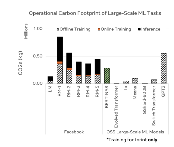
Comprehensive carbon accounting methodologies
AI’s impact extends beyond operational energy consumption. Comprehensive carbon footprint assessment integrates the Three-Phase Lifecycle Analysis (training, inference, manufacturing) with the three standard emission scopes defined by the GHG Protocol. With AI projected to grow rapidly through 2030, understanding total lifecycle costs across all phases and scopes is essential for identifying the most impactful sustainability interventions.
Within an owned data-center facility boundary, Scope 1 emissions originate from on-site power generation including backup diesel generators, facility cooling systems, and owned power plants. While many AI data centers primarily use grid electricity, those with fossil-fuel backup systems or owned generation contribute directly to emissions.
Scope 2 emissions represent indirect emissions from electricity purchased to power AI infrastructure. This is often the dominant category for owned facility operations, and it varies dramatically by geographic location and grid energy mix. As established in our geographic optimization discussion, training location can create up to 75\(\times\) differences in carbon intensity.
Scope 3 emissions constitute the most complex category, encompassing hardware manufacturing, cloud supply chains, transportation, disposal, and downstream use. Semiconductor manufacturing is carbon-intensive.25 Producing a single high-performance AI accelerator generates emissions equivalent to several years of operational energy use. Under company-wide or value-chain AI accounting, Scope 3 can dominate even when Scope 2 dominates a single owned facility’s operational footprint.
25 EUV Lithography Energy Cost: Each ASML EUV machine draws 1 MW continuously and consumes 30,000 liters of ultrapure water daily, a 10\(\times\) energy increase over older deep-UV systems. Since EUV is required for sub-7 nm nodes used in every modern AI accelerator, the embodied energy of each chip generation compounds: more transistors per die means more EUV exposure steps, making advanced-node fabrication an irreducible and growing component of AI’s Scope 3 emissions.
26 Edge AI Energy Paradox: Edge inference reduces per-query latency from 100–200 ms (cloud) to 1–10 ms, but distributes power draw across many always-on devices. Tesla’s FSD computer draws 72 W continuously while driving; scaling comparable onboard compute across a global vehicle fleet would imply roughly 100 GW of collective power, comparable to dozens of large power plants. The sustainability trade-off is that edge eliminates network energy but creates an unmetered, distributed energy footprint invisible to carbon accounting frameworks.
Beyond manufacturing, Scope 3 emissions include the downstream impact of AI once deployed. AI services such as search engines, social media platforms, and cloud-based recommendation systems operate at enormous scale, requiring continuous inference across millions or even billions of user interactions. The cumulative electricity demand of inference workloads can ultimately surpass the energy used for training, further amplifying AI’s carbon impact. End-user devices, including smartphones, IoT devices, and edge computing26 platforms, also contribute to Scope 3 emissions, as their AI-enabled functionality depends on sustained computation. Companies such as Meta and Google report that Scope 3 emissions from AI-powered services make up the largest share of their total environmental footprint, due to the sheer scale at which AI operates.
Operational emissions capture only the production phase of AI. Software development itself adds another layer of environmental impact that is rarely accounted for.
The GHG Protocol27 framework (Institute and Sustainable Development 2023) provides the standard categorization for these emissions. Figure 15 illustrates the three scopes:
27 GHG Protocol: Developed jointly by the World Resources Institute and WBCSD, this framework is used by over 90 percent of Fortune 500 companies reporting to CDP. Its three-scope taxonomy matters for ML systems because most AI carbon hides in Scope 3 (hardware manufacturing, cloud compute supply chains), which companies historically underreport by 50–70 percent compared to Scopes 1 and 2.
Institute, World Resources, and World Business Council for Sustainable Development. 2023. Greenhouse Gas Protocol: Corporate Standard.
- Scope 1 (Direct Emissions): Arise from direct company operations—backup generators, company-owned power generation.
- Scope 2 (Indirect Energy Emissions): Electricity purchased from the grid, the primary emission source for cloud computing workloads.
- Scope 3 (Value Chain Emissions): Extend beyond direct control—semiconductor manufacturing, hardware transportation, end-of-life disposal of AI accelerators.

Categorizing these emissions into Scope 1, 2, and 3 frameworks provides a standardized vocabulary for corporate environmental reporting. Correctly applying this framework in practice requires classifying the various hidden emission sources across a typical ML platform’s operational lifecycle.
Checkpoint 1.3: Accounting for invisible carbon
You are auditing the carbon footprint of a Machine Learning platform. Classify the following emission sources into Scope 1 (Direct), Scope 2 (Indirect Energy), or Scope 3 (Value Chain):
- Diesel burned by backup generators during a grid outage at your owned facility.
- Electricity purchased from the grid to power your leased NVIDIA H100 cluster.
- The embodied carbon emitted during the manufacturing of the GPUs by TSMC.
- Emissions from the end-user’s smartphone battery while running your mobile inference app.
Accurately classifying these hidden emissions forces engineering teams to take responsibility for the entire value chain of their deployments. The comprehensive accounting framework also reveals that the dominant share of energy shifts once a model moves from the training phase to global inference.
Self-Check: Question
A facility engineer is redesigning a datacenter aisle to host training racks after hosting web-serving racks for a decade. Which property of AI workloads most forces the redesign, relative to a typical web stack?
- AI workloads demand sub-millisecond tail latency that web stacks do not, so racks must be packed less densely to keep idle spares available.
- AI training holds large numbers of accelerators near peak utilization for weeks, creating sustained thermal density and power draw rather than the bursty CPU spikes web stacks produce.
- AI workloads use less energy per request than web traffic, so the real change is accounting rules rather than physical design.
- AI workloads avoid cooling needs because regular matrix arithmetic produces less heat than irregular web request patterns.
A team consolidates training jobs from a fleet at 45 percent average utilization onto a smaller active cluster at 85 percent utilization, powering down the drained nodes. Explain why this yields a sustainability win even if no model becomes more accurate, and state what part of the section’s total-energy model it targets.
A team doubles the number of GPUs in a distributed training job, expecting roughly linear energy scaling. Instead, they observe networking energy growing much faster than 2x. Which mechanism does the section identify as the primary cause, and what sustainability risk does it create?
- Total arithmetic decreases, so the model has to train longer to recover lost FLOPs, raising total energy.
- AllReduce and all-to-all gradient synchronization scale worse than linearly with cluster size and can add 20 to 40 percent to total energy, making naive cluster-size scaling carbon-inefficient.
- Facility PUE automatically worsens in direct proportion to node count regardless of cooling design.
- Embodied carbon per chip vanishes once a model is split across enough nodes, masking the true energy cost.
You are auditing carbon accounting for a team running training on a leased GPU cluster. The team reports five emissions sources as shown. Which classification across the GHG Protocol scopes is correct?
S1: Diesel burned by backup generators the team owns on-site. S2: Electricity purchased from the grid to power the leased GPUs. S3: Cooling electricity drawn inside the same datacenter. S4: The embodied carbon from manufacturing the accelerators themselves. S5: Energy used by end-user phones that run the deployed model.
- S1 Scope 1; S2 Scope 2; S3 Scope 2; S4 Scope 3; S5 Scope 3.
- S1 Scope 2; S2 Scope 1; S3 Scope 3; S4 Scope 3; S5 Scope 2.
- S1 Scope 3; S2 Scope 3; S3 Scope 2; S4 Scope 1; S5 Scope 1.
- S1 Scope 1; S2 Scope 1; S3 Scope 1; S4 Scope 2; S5 Scope 2.
Which example is most clearly Scope 3 in the chapter’s accounting framework rather than Scope 1 or Scope 2?
- Diesel burned by backup generators owned by the datacenter operator.
- Grid electricity purchased to power a leased GPU cluster.
- Cooling electricity consumed inside the datacenter and billed on the same meter as compute.
- Embodied carbon from manufacturing accelerators plus downstream energy used by end-user devices running the deployed service.
Training vs. Inference Energy Analysis
Training a massive language model is a spectacular, highly visible energy event, akin to launching a rocket. Deploying that same model to serve a billion daily queries is like operating an international airline fleet. Training burns thousands of megawatt-hours in a single, concentrated burst over several months; inference burns energy continuously, query by query, year after year. Understanding where the majority of the energy budget goes dictates where optimization efforts must concentrate.
Optimization opportunities differ across lifecycle phases. Training optimizations focus on computational efficiency and hardware utilization, while inference optimizations emphasize latency, throughput, and edge deployment strategies. Matching the sustainability intervention to the dominant energy consumer for each application yields the greatest returns.
Training energy demands
Training frontier AI models requires computational infrastructure with hundreds of thousands of cores and specialized AI accelerators operating continuously for months. Microsoft’s 2020 disclosure of the OpenAI dedicated supercomputer, built specifically for large-scale AI training at the time, reported 285,000 CPU cores, 10,000 GPUs, and network bandwidth exceeding 400 gigabits per second per server (Patterson et al. 2021). Frontier infrastructure has since grown more than an order of magnitude; this 2020 figure remains useful as a calibrated reference point rather than a current frontier number.
The intensive computational loads generate heat that cooling infrastructure must continuously remove, adding 30–40 percent to total energy requirements. Reducing this overhead requires co-optimization of hardware architecture, parallelism strategy, and algorithmic efficiency.
Training energy costs occur once per model. The primary sustainability challenge emerges during deployment, where inference workloads continuously serve millions or billions of users.
Inference energy costs
Inference workloads execute every time an AI model responds to queries, classifies images, or makes predictions. Unlike training, inference scales dynamically and continuously across applications such as search engines, recommendation systems, and generative AI models. Although each individual inference request consumes far less energy compared to training, the cumulative energy usage from billions of daily AI interactions quickly surpasses training-related consumption (Patterson et al. 2021).
For example, AI-driven search engines handle billions of queries per day, recommendation systems provide personalized content continuously, and generative AI services such as ChatGPT or DALL-E have substantial per-query computational costs. The inference energy footprint is high in transformer-based models due to high memory and computational bandwidth requirements.
McKinsey’s then-forward-looking market analysis for inference workloads projected dramatic growth. Figure 16 tracks data center inference from $4–5 billion in 2017 to a projected $9–10 billion by 2025, more than doubling in size. Similarly, edge inference workloads were projected to increase from less than $0.1 billion to $4–4.5 billion in the same period. This growth substantially outpaced the projected expansion of training workloads in both environments, highlighting how the economic footprint of inference was expected to outgrow that of training operations.

Unlike traditional software applications with fixed energy footprints, inference workloads dynamically scale with user demand. AI services like Alexa, Siri, and Google Assistant rely on continuous cloud-based inference, processing millions of voice queries per minute, necessitating uninterrupted operation of energy-intensive data center infrastructure.
The energy inefficiency of the decode phase
The energy gap between the two inference phases is striking (Figure 17).

The prefill/decode distinction summarized in Prefill vs. Decode Characteristics extends beyond latency into energy efficiency. Recent analysis (Ma et al. 2026) reveals that autoregressive generation is inherently energy-wasteful compared to batch processing.
Ma, Yufei, Sayak Pawar, Aayush Cherian, Pramod Khargonekar, Saurabh Patel, Michael Pellauer, and Joel S. Emer. 2026. Challenges and Research Directions for Large Language Model Inference Hardware.
- Prefill (Compute-Bound): High arithmetic intensity allows the GPU to perform thousands of operations for every byte read from memory, achieving near-peak energy efficiency (pJ/FLOP).
- Decode (Bandwidth-Bound): The “Decode” phase requires reading the entire model weight set from HBM to generate a single token. Since arithmetic intensity is low, the compute units sit idle for much of the cycle.
The result is Static Power Waste: the GPU draws significant leakage and clock power while waiting for memory transfers. Generating 1,000 tokens through 1,000 sequential decode steps can therefore consume 10–50\(\times\) more energy than processing the same 1,000 tokens in a single prefill batch. The inefficiency drives demand for specialized, memory-optimized NPUs and TPUs examined in Compute Infrastructure, which prioritize bandwidth-per-watt over raw TFLOPS.
Edge AI impact
The edge intelligence architectures from Edge Intelligence enable inference beyond centralized data centers. This distributed approach offers unique sustainability advantages by reducing data transmission energy costs and lowering dependency on high-power cloud infrastructure. Instead of routing every AI request to centralized cloud servers, models can be deployed directly on user devices or at edge computing nodes.
However, running inference at the edge does not eliminate energy concerns, especially when AI is deployed at scale. Autonomous vehicles, for instance, require millisecond-latency AI inference, meaning cloud processing is impractical. Instead, vehicles are now being equipped with onboard AI accelerators that function as “data centers on wheels” (Sudhakar et al. 2023). These embedded computing systems process real-time sensor data equivalent to small data centers, consuming significant power even without relying on cloud inference.
Sudhakar, Soumya, Vivienne Sze, and Sertac Karaman. 2023. “Data Centers on Wheels: Emissions from Computing Onboard Autonomous Vehicles.” IEEE Micro 43 (1): 29–39. https://doi.org/10.1109/mm.2022.3219803.
Similarly, consumer devices such as smartphones, wearables, and IoT sensors individually consume milliwatts to watts of power but collectively add terawatt-hours to global energy use due to their sheer numbers. Therefore, the efficiency benefits of edge computing must be balanced against the extensive scale of device deployment.
Edge deployment can be more sustainable than cloud deployment when designed correctly. The combination of eliminated data transmission, local processing efficiency, and duty-cycled operation can reduce total system energy consumption by orders of magnitude compared to always-connected cloud inference.
Edge and mobile power budgets
ARM-based edge devices operate under fundamentally different power constraints than data center GPUs. Understanding these constraints is essential for sustainable edge AI system design:
Power budgets reflect the physical constraints of battery capacity, thermal dissipation, and deployment environment. Table 5 shows how these constraints propagate: TinyML devices operating from coin cells or energy harvesting cannot exceed milliwatt average power, mobile devices must balance user experience with battery life, and automotive systems face thermal constraints within enclosed vehicle compartments despite having access to vehicle power.
| Platform Category | Idle Power | Active Power | Peak Power | Example Devices |
|---|---|---|---|---|
| TinyML (MCU) | 1–100 W | 1–50 mW | 100 mW | Arduino Nano 33, STM32H7, Nordic nRF5340 |
| Mobile NPU | 10-100 mW | 0.5–5 W | 10 W | Pixel Tensor, Apple Neural Engine, Snapdragon NPU |
| Edge GPU/TPU | 1-5 W | 5–30 W | 75 W | NVIDIA Jetson Orin NX (10–25 W) and AGX Orin (15–60 W), Google Edge TPU, RPi AI Kit |
| Autonomous Vehicle | 10–50 W | 50–200 W | 500 W | Tesla FSD Computer, Mobileye EyeQ, NVIDIA Drive |
TinyML power state dynamics
While Edge Intelligence examines TinyML from a systems architecture perspective, the energy efficiency of on-device inference is equally a sustainability consideration: each of the billions of edge inference calls aggregates into measurable carbon footprint at fleet scale. TinyML efficiency depends heavily on duty cycling, where devices alternate between deep sleep and active inference. Equation 14 expresses average power as a weighted sum of active and sleep power:
\[P_{\text{average}} = P_{\text{active}} \times \frac{t_{\text{inference}}}{T_{\text{period}}} + P_{\text{sleep}} \times \frac{T_{\text{period}} - t_{\text{inference}}}{T_{\text{period}}} \tag{14}\]
For a keyword-spotting model running on a Cortex-M4 microcontroller (Archetype C (Federated MobileNet) regime, Three systems archetypes):
- Active inference power: 15 mW for 20 ms per detection cycle
- Deep sleep power: 10 microamps at 3.3V (33 microwatts)
- Detection period: 1 second (continuous listening)
\[P_{\text{average}} = 15 \text{ mW} \times \frac{20 \text{ ms}}{1000 \text{ ms}} + 0.033 \text{ mW} \times \frac{980 \text{ ms}}{1000 \text{ ms}}\]
\[P_{\text{average}} = 0.30 \text{ mW} + 0.032 \text{ mW} = 0.33 \text{ mW}\]
At this average power, a 250 mAh coin cell battery (at 3.0V nominal) provides approximately 2,270 hours of operation, nearly 95 days of continuous always-on AI inference. This calculation demonstrates how TinyML enables sustainable AI deployment scenarios impossible with higher-power platforms.
These power-aware design principles carry directly into practical industrial deployment scenarios.
Example 1.3: Battery life for TinyML
Consider deploying an anomaly detection model on a factory sensor node:
System parameters:
- Model: Autoencoder for vibration anomaly detection
- MCU: ARM Cortex-M4 at 80 MHz
- Inference latency: 5 ms per sample
- Sampling rate: 10 Hz (100 ms period)
- Active power: 12 mW during inference
- Sleep power: 5 microamps at 3.3V (16.5 microwatts)
- Battery: two AA cells (3000 mAh at 3.0V)
Step 1: Calculate duty cycle and average power. \[D = \frac{5 \text{ ms}}{100 \text{ ms}} = 0.05 \text{ (5\% duty cycle)}\]
\[P_{\text{avg}} = 12 \text{ mW} \times 0.05 + 0.0165 \text{ mW} \times 0.95 = 0.60 + 0.016 = 0.616 \text{ mW}\]
Step 2: Calculate battery life. \[E_{\text{battery}} = 3000 \text{ mAh} \times 3.0 \text{ V} = 9000 \text{ mWh}\]
\[t_{\text{life}} = \frac{9000 \text{ mWh}}{0.616 \text{ mW}} = 14,610 \text{ hours} \approx 1.7 \text{ years}\]
The deployment achieves continuous AI-powered monitoring for nearly two years on standard batteries, demonstrating the sustainability potential of TinyML systems designed with power-aware principles.
On-device learning and the battery wall
While inference on TinyML devices is highly efficient, on-device learning introduces a much steeper energy challenge. Personalizing a model to a user’s specific voice or gait requires backpropagation, which demands 2–3\(\times\) more compute and memory than forward inference.
The thermal design power (TDP) of mobile processors creates hard constraints that shape every aspect of on-device learning strategies. Modern smartphones typically maintain sustained processing at 2–3 W for ML workloads to prevent thermal discomfort, but can burst to 5–10 W for brief periods before thermal throttling occurs. This thermal design power determines the entire feasible space of adaptive algorithms.
Napkin Math 1.5: The energy of learning
Problem: Consider fine-tuning a small language model (1B parameters) on a user’s smartphone overnight. Is this feasible within a 5 percent battery budget?
Math:
- Phone Battery: Typical capacity is approximately 12.5 Wh (Watt-hours), or about 45,000 Joules.
- Budget: 5 percent of 45,000 J = 2,250 Joules.
- Training Cost:
- Forward pass: \(\approx\) 2 nJ/param.
- Backward pass: \(\approx\) 4 nJ/param.
- Total per token: 6 nJ/param \(\times 10^9\) params = 6 Joules/token.
- Capacity: 2,250 J / 6 J/token = 375 tokens.
Systems insight: Full fine-tuning is impossible within a reasonable daily battery budget. Sustainable on-device learning requires PEFT (Parameter-Efficient Fine-Tuning) or sparse updates to reduce the energy cost per token by 100\(\times\) or more.
The fundamental physics of energy consumption reveals why local processing is almost always preferable to cloud offloading for on-device learning, provided the model is sufficiently compact.
Systems Perspective 1.4: The energy hierarchy
Trade-off: The architectural choice between processing data locally and sending it to the cloud is governed by an energy budget. The physics of energy consumption provides a clear answer based on the Energy-to-Communication Ratio.
Energy cost per operation (approximate):
- 32-bit Integer Add: 0.1 pJ
- 32-bit Float Mult: 4.0 pJ
- Wireless Transmit (1 bit): 100,000–500,000 pJ (Bluetooth/WiFi)
Systems insight: Transmitting a single bit of data costs roughly the same energy as performing 25,000 to 125,000 FP32 multiplies, or 1 million to 5 million 32-bit integer adds, under these operation-cost assumptions. When insight can be extracted from data using fewer than roughly 100,000 floating-point operations per bit, local processing is usually more energy efficient than cloud offloading. This ratio drives the architecture of federated learning: compute is cheap; radio transmission is expensive.
Energy harvesting for autonomous edge AI
With sufficient optimization, TinyML enables energy-autonomous operation where devices harvest ambient energy rather than relying on batteries:
Consider Table 6: a keyword spotting model optimized to 0.5 mW average power can operate indefinitely on approximately 5 square centimeters of indoor solar harvesting only under bright indoor conditions near the top of the listed range. Typical indoor deployments need additional area, energy storage, duty cycling, or a lower average-power model to leave margin for conversion losses and dim lighting. This perpetual operation model represents the ultimate sustainable edge AI deployment, where operational energy comes entirely from ambient sources.
| Harvesting Source | Typical Power | Viable TinyML Applications |
|---|---|---|
| Indoor solar (1 cm^2) | 10-100 microwatts | Periodic sensor classification |
| Outdoor solar (1 cm^2) | 1-10 milliwatts | Continuous keyword spotting |
| Thermoelectric (body heat) | 10-100 microwatts | Wearable gesture recognition |
| RF harvesting (WiFi) | 1-10 microwatts | Ultra-low-duty sensor nodes |
| Vibration piezoelectric | 100 microwatts-1 mW | Industrial monitoring |
Sustainable edge deployment patterns
Beyond individual device efficiency, architectural patterns determine total system energy consumption across edge-cloud boundaries:
Cascade inference architecture
Deploy a small edge model (under 100 KB) to filter inputs before cloud inference. Equation 15 expresses total energy as the sum of local processing plus probabilistically-triggered cloud costs:
\[E_{\text{cascade}} = E_{\text{edge}} + p_{\text{escalate}} \times (E_{\text{transmit}} + E_{\text{cloud}}) \tag{15}\]
where \(p_{\text{escalate}}\) is the probability of requiring cloud inference (typically 5–20 percent for well-designed cascades).
For a visual inspection system:
- Edge model (MobileNet-v3 tiny): 0.5 mJ per image classification
- Cloud model (ResNet-152): 50 mJ per classification
- Transmission energy: 10 mJ per image (cellular)
- Escalation rate: 10 percent (only ambiguous cases sent to cloud)
\[E_{\text{cascade}} = 0.5 + 0.10 \times (10 + 50) = 0.5 + 6.0 = 6.5 \text{ mJ/image}\]
Compared to always-cloud inference at 60 mJ per image, the cascade architecture achieves 89 percent energy reduction while maintaining accuracy through selective cloud escalation.
Wake-word triggered systems
Always-on systems use hierarchical wake detection to minimize average power:
- Ultra-low-power analog front end: 10 microwatts continuous voice activity detection
- Tiny neural network wake detector: 100 microwatts when speech detected
- Full model inference: 10 mW for 50 ms when wake word confirmed
With typical speech activity rates of 5 percent and wake word occurrence of 0.1 percent:
\[P_{\text{average}} = 0.01 + 0.05 \times 0.1 + 0.001 \times 10 \times 0.05 = 0.0155 \text{ mW}\]
The hierarchical approach achieves 15.5 microwatts average power compared to 10 mW for always-active full inference, a 645\(\times\) reduction enabling battery-powered voice assistants with multi-year operation.
Federated learning energy analysis
Training at the edge eliminates data transmission but increases local compute. Equation 16 contrasts the energy trade-offs between federated and centralized approaches:
\[E_{\text{federated}} = N \times E_{\text{local\_train}} + E_{\text{aggregation}}\] \[E_{\text{centralized}} = N \times E_{\text{transmit}} + E_{\text{cloud\_train}} \tag{16}\]
Federated learning becomes more energy-efficient when data sizes exceed model update sizes. For privacy-sensitive applications with rich sensor data, federated approaches often achieve both privacy and energy benefits, as transmitting model weight updates (megabytes) requires less energy than transmitting raw data (gigabytes) for applications like on-device personalization.
AI’s environmental footprint extends beyond electricity consumption to include physical resources—water, hazardous chemicals, and critical materials—that require different assessment approaches.
Resource consumption and ecosystem effects
Carbon footprint analysis provides a crucial but incomplete picture of AI’s environmental impact. Comprehensive assessment requires measuring additional ecological impacts including water consumption, hazardous chemical usage, rare material extraction, and biodiversity disruption that often receive less attention despite their ecological significance. Modern semiconductor fabrication plants producing AI chips require millions of liters of water daily and use over 250 hazardous substances in their processes. In regions already facing water stress, such as Taiwan, Arizona, and Singapore, this intensive usage threatens local ecosystems and communities. AI hardware also relies heavily on scarce materials like gallium, indium, arsenic, and helium, which face both geopolitical supply risks and depletion concerns (Jha 2014; Chen 2006). These resource dependencies are examined in detail in the hardware lifecycle assessment that follows.
Jha, A. R. 2014. Rare Earth Materials: Properties and Applications. CRC Press. https://doi.org/10.1201/b17045.
Chen, H.-W. 2006. “Gallium, Indium, and Arsenic Pollution of Groundwater from a Semiconductor Manufacturing Area of Taiwan.” Bulletin of Environmental Contamination and Toxicology 77 (2): 289–96. https://doi.org/10.1007/s00128-006-1062-3.
Water, chemicals, and critical materials
Semiconductor fabrication is an exceptionally water-intensive process (Cooper et al. 2011). TSMC’s fab in Arizona is projected to consume 34 million liters of water per day28 (Reuters 2024), accounting for nearly 3 percent of the city’s total water production. A single 300mm silicon wafer requires over 8,300 liters of water throughout the complete fabrication process. Figure 18 illustrates the typical fab water cycle, where advanced recycling can reclaim 60–80 percent of water but still leaves a substantial consumption footprint.
Cooper, Tom, Suzanne Fallender, Joyann Pafumi, Jon Dettling, Sebastien Humbert, and Lindsay Lessard. 2011. “A Semiconductor Company’s Examination of Its Water Footprint Approach.” Proceedings of the 2011 IEEE International Symposium on Sustainable Systems and Technology, 1–6. https://doi.org/10.1109/issst.2011.5936865.
28 Semiconductor Water Scale: TSMC’s Arizona fab will consume 12 billion liters annually (about 4,800 Olympic pools), and advanced-node AI chips require 5–10\(\times\) more water per die than older process nodes due to additional EUV and cleaning steps. This water dependency creates a direct sustainability constraint: fabs compete with municipal water supplies in drought-prone regions like Arizona and Taiwan, where semiconductor water demand can reach 3 percent of a city’s total allocation.
Reuters. 2024. Water-Guzzling Chipmaker TSMC and Drought-Plagued Arizona Are an Unlikely Pair, but Phoenix Says It Has Enough Water. Fortune magazine, 8 April 2024.

The critical takeaway from Figure 18 is that even with 60–80 percent reclamation rates, the absolute volume of ultra-pure water consumed by advanced-node fabs remains enormous, creating a hard physical constraint on where AI chip manufacturing can sustainably operate.
Fabrication is also heavily reliant on hazardous chemicals for etching, doping, and cleaning. Strong acids (hydrofluoric, sulfuric), volatile organic compounds like xylene, and highly toxic gases (arsine, phosphine) are used in massive quantities—a large fab may consume over 2,000 metric tons of acids annually (Kim et al. 2018). These substances create hazardous waste streams requiring extensive treatment to prevent ecological harm.
Kim, Sunju, Chungsik Yoon, Seunghon Ham, Jihoon Park, Ohun Kwon, Donguk Park, Sangjun Choi, Seungwon Kim, Kwonchul Ha, and Won Kim. 2018. “Chemical Use in the Semiconductor Manufacturing Industry.” International Journal of Occupational and Environmental Health 24 (3-4): 109–18. https://doi.org/10.1080/10773525.2018.1519957.
Davies, Martin. 2011. “Endangered Elements: Critical Thinking.” Critical Thinking in Study Skills for International Postgraduates. Macmillan Education UK. https://doi.org/10.1007/978-0-230-34553-9_8.
AI hardware depends on a suite of scarce and geopolitically sensitive critical materials. While silicon is abundant, high-performance chips require rare elements like gallium, indium, tantalum, and helium. Materials such as indium appear on critical-materials lists under reserve, substitution, and supply-risk analyses (Davies 2011). The geographic concentration of rare earth refining creates significant supply chain vulnerabilities. Table 7 quantifies the scope of this material dependency challenge.
| Material | Application in AI Semiconductor Manufacturing | Supply Concerns |
|---|---|---|
| Silicon (Si) | Primary substrate for chips, wafers, transistors | • Processing constraints • Geopolitical risks |
| Gallium (Ga) | GaN-based power amplifiers, high-frequency components | • Limited availability • Byproduct of aluminum and zinc production |
| Germanium (Ge) | High-speed transistors, photodetectors, optical interconnects | • Scarcity • Geographically concentrated |
| Indium (In) | Indium Tin Oxide (ITO), optoelectronics | • Limited reserves • Recycling dependency |
| Tantalum (Ta) | Capacitors, stable integrated components | • Conflict mineral • Vulnerable supply chains |
| Rare Earth Elements (REEs) | Magnets, sensors, high-performance electronics | • High geopolitical risks • Environmental extraction concerns |
| Cobalt (Co) | Batteries for edge computing devices | • Human rights issues • Geographical concentration (Congo) |
| Tungsten (W) | Interconnects, barriers, heat sinks | • Limited production sites • Geopolitical concerns |
| Copper (Cu) | Interconnects, barriers, heat sinks | • Limited high-purity sources • Geopolitical concerns |
| Helium (He) | Semiconductor cooling, plasma etching, EUV lithography | • Nonrenewable • Irretrievable atmospheric loss • Limited extraction capacity |
The construction and operation of fabs and data centers also directly impacts natural ecosystems through habitat destruction, water stress from aquifer depletion, and pollution from chemical discharge. In Hsinchu, Taiwan, extensive water extraction by fabs has led to falling water tables and seawater intrusion, affecting both agriculture and aquatic biodiversity (Hsu et al. 2016). Waste generation from fabrication—including gaseous emissions, VOC-laden air, and metal-contaminated wastewater—requires advanced treatment systems, and the end-of-life disposal of AI hardware contributes to a growing e-waste crisis, with only 17.4 percent of global e-waste properly recycled (Singh and Ogunseitan 2022).
Hsu, Liang-Ching, Ching-Yi Huang, Yen-Hsun Chuang, Ho-Wen Chen, Ya-Ting Chan, Heng Yi Teah, Tsan-Yao Chen, Chiung-Fen Chang, Yu-Ting Liu, and Yu-Min Tzou. 2016. “Accumulation of Heavy Metals and Trace Elements in Fluvial Sediments Received Effluents from Traditional and Semiconductor Industries.” Scientific Reports 6 (1): 34250. https://doi.org/10.1038/srep34250.
The environmental toll of our computational demands extends far beyond atmospheric carbon, manifesting as severe water stress and ecological disruption around manufacturing hubs. This sobering reality converges on the ultimate physical consequence of the AI arms race: the disposition of massive, resource-intensive hardware clusters that become obsolete within three years.
Self-Check: Question
A model costs 1,287 MWh to train once and then serves 10 million queries per day at 0.001 kWh per query for a five-year product life. Which explanation best captures why inference often dominates lifecycle energy for widely deployed models?
- Inference always uses more power per operation than training because of serving-specific hardware.
- The model must be retrained on every query once in production, so inference and retraining overlap.
- Inference runs continuously across enormous cumulative query volume — here, about 10 MWh per day — so after roughly 130 days the cumulative serving energy matches the one-time training run, and after five years it dwarfs it.
- Inference cannot use specialized accelerators, unlike training, so it draws more grid power per step.
A profiler shows that the decode phase of an LLM serving stack sustains only 6 percent of peak FP16 TFLOPS while HBM bandwidth sits near 90 percent utilization and static power keeps flowing. Which mechanism does the section identify as the dominant source of decode energy inefficiency, and what does it imply for optimization?
- Decode disables on-chip caches, so all work shifts to the CPU and server-class RAM.
- Decode is memory-bandwidth-bound — each token requires reading the model’s weights while the compute units idle — so the accelerator burns static power without producing proportional useful work; the fix is to reduce bytes read through quantization, smaller KV caches, or weight fusion.
- Prefill uses lower numerical precision while decode must always use FP32, so decode pays a precision tax.
- Decode inefficiency comes from a transient rise in facility PUE during serving hours.
A product manager claims that moving inference from the cloud to 50 million edge devices automatically solves the deployment’s sustainability problem. Explain why the chapter considers this claim incomplete and identify the lifecycle terms the edge decision can actually shift.
A keyword-spotting sensor runs 10 ms of active inference once per second and sleeps the remaining 990 ms at microwatt draw. Active power is 120 mW; sleep power is 50 uW. Which quantity most strongly determines the device’s average power, per the section’s duty-cycle reasoning?
- The duty cycle, because 0.010 / 1.000 x 120 mW plus (0.990 / 1.000 x 0.050 mW) is roughly 1.25 mW — the active burst dominates this average, but the low duty cycle keeps power far below continuous 120 mW operation.
- The datacenter’s hourly carbon intensity, because the sensor uploads to a cloud pipeline.
- The model’s total parameter count, because larger models always consume more per-second energy.
- Whether the model was distilled from a larger teacher, because distillation changes average power directly.
A startup wants to support nightly on-device full fine-tuning of a 1B-parameter model on consumer smartphones. Explain why the chapter argues this is infeasible within a realistic overnight battery budget and which class of methods it recommends instead.
Order the following stages in a hierarchical wake-word cascade designed to minimize average power on a battery-powered smart speaker: (1) full large-model inference on the captured utterance, (2) ultra-low-power voice-activity detection running continuously at microwatts, (3) small neural wake-word detector running only when voice is present.
Hardware Lifecycle and E-Waste
The environmental cost of an AI accelerator begins long before its first FLOP is calculated (Harris 2023). The embodied carbon of a single NVIDIA H100 GPU is estimated at 150 to 200 kg of CO2 equivalent from manufacturing alone.29 The fleet of thousands of such processors required to train our 175B parameter model—consuming 1,287 MWh of electricity—represents a significant upfront carbon investment before any computation occurs. A comprehensive Life Cycle Assessment (LCA) quantifies the cumulative environmental impact across four key phases: design, manufacture, use, and disposal. LCA reveals that hardware manufacturing often contributes 30–50 percent of an AI system’s total lifetime emissions, making it a critical sustainability lever that operational efficiency improvements alone cannot address.
Harris, M. 2023. “The Environmental Cost of Next-Generation AI Chips: Energy, Water, and Carbon Impacts.” Journal of Green Computing 17 (1): 22–38.
29 Life Cycle Assessment (LCA): Standardized by ISO 14040/14044 in the 1990s, LCA traces environmental impact from raw material extraction through disposal. For AI hardware, LCA consistently reveals that manufacturing contributes 30–50 percent of total lifetime emissions, a share that grows as operational energy shifts to renewables. This makes hardware refresh cycles and accelerator lifespan extension first-order sustainability levers that operational efficiency alone cannot substitute.
Checkpoint 1.4: The training-inference flip
Consider a vision model where training requires 2,000 GPU-hours at an average power draw of 300 W. Once deployed, the model serves 1 million requests per day, with each request taking 50 ms at an average draw of 100 W.
- Calculate the total energy used for training.
- Calculate the total energy used for inference over a 2-year product lifespan.
- Determine the “Inference-to-Training Ratio.” Based on this, where should an engineer focus optimization efforts to maximize sustainability?
Life Cycle Assessments reveal that discarding functional hardware purely for modest efficiency gains often causes more environmental harm through embodied carbon than it saves in operational power. To mathematically evaluate the tipping point where new hardware becomes environmentally justified, we must calculate the exact intersection of training costs, inference scale, and hardware lifespans.
Each of the four primary lifecycle stages contributes to an AI system’s total environmental footprint. Figure 19 visualizes this progression from design through disposal, highlighting the interdependencies between phases and the environmental impact categories associated with each stage.

Design and experimentation phase
The design phase encompasses the research, development, and optimization of ML models before deployment—iterating on architectures, tuning hyperparameters, and running training experiments. The environmental cost of this phase is often underestimated because reported training energy (such as GPT-3’s 1,287 MWh) reflects only the final run, not the extensive trial-and-error that preceded it. Automated architecture search techniques evaluate hundreds or thousands of configurations, each requiring a separate training cycle. Early neural architecture search (NAS) required 1,800 GPU-days; efficient variants like DARTS reduce this to 1–4 GPU-days through weight-sharing and differentiable search (Strubell et al. 2019). Table 8 reveals stark differences in emissions across model scales.
| AI Model | Training FLOPs | Estimated CO2 Emissions (kg) | Equivalent Car Distance |
|---|---|---|---|
| GPT-3 | \(3.1 \times 10^{23}\) | 502,000 kg | 1.9 million km |
| T5-11B | \(2.3 \times 10^{22}\) | 85,000 kg | 338,000 km |
| BERT (Base) | \(3.3 \times 10^{18}\) | 650 kg | 2,400 km |
| ResNet-50 | \(2.0 \times 10^{17}\) | 35 kg | 129 km |
Addressing the design phase’s sustainability challenges requires innovations in training efficiency: sparse training, low-precision arithmetic, weight-sharing, and energy-aware NAS approaches. Transfer learning and fine-tuning pretrained models can reduce computational costs by orders of magnitude compared to training from scratch (Gupta et al. 2022).
Gupta, U., M. Elgamal, G. Hills, G.-Y. Wei, H.-H. S. Lee, D. Brooks, and C.-J. Wu. 2022. “Act: Designing Sustainable Computer Systems with an Architectural Carbon Modeling Tool.” Proceedings of the 49th Annual International Symposium on Computer Architecture, 784–99. https://doi.org/10.1145/3470496.3527408.
Manufacturing phase
The manufacturing of AI hardware is enormously resource-intensive, with the embodied carbon of a single H100 GPU reaching 150–200 kg CO2 equivalent before any computation occurs. Semiconductor fabrication requires extreme precision through processes such as EUV lithography—each tool consuming approximately 1 MW of continuous power—chemical vapor deposition, and ion implantation. The resource demands detailed in Section 1.5.3 reveal the scale: TSMC’s Arizona fab consumes 34 million liters of water daily, fabrication relies on over 250 hazardous substances, and the supply chain depends on geopolitically concentrated critical materials.
The energy required to manufacture AI hardware is substantial, with the total energy cost per chip often exceeding its entire operational lifetime energy use in clean-grid regions. A single 5nm fabrication plant consumes millions of liters of ultrapure water daily and relies on energy-intensive processes that generate significant CO2 emissions. Recognizing these challenges, industry leaders including Intel, TSMC, and Samsung have pledged to transition toward carbon-neutral fabrication through renewable energy integration, closed-loop water recycling systems, and eco-friendly etching techniques that minimize hazardous waste generation (Cenci et al. 2021; Irimia-Vladu 2014).
Cenci, Marcelo Pilotto, Tatiana Scarazzato, Daniel Dotto Munchen, Paula Cristina Dartora, Hugo Marcelo Veit, Andrea Moura Bernardes, and Pablo R. Dias. 2021. “Eco-Friendly Electronics—a Comprehensive Review.” Advanced Materials Technologies 7 (2): 2001263. https://doi.org/10.1002/admt.202001263.
Irimia-Vladu, M. 2014. “‘Green’ Electronics: Biodegradable and Biocompatible Materials and Devices for Sustainable Future.” Chem. Soc. Rev. 43 (2): 588–610. https://doi.org/10.1039/c3cs60235d.
Use phase
The operational energy consumed during training and inference is detailed in Section 1.5. What merits attention here is the pattern of this consumption and its interaction with grid infrastructure. The 1,287 MWh required to train our 175B model represents a massive, inflexible power draw that runs 24/7, making it difficult to shift workloads to times of higher renewable energy availability.
The inflexibility exacerbates a critical grid management problem known as the duck curve—as solar power ramps down in the late afternoon, grid operators must rapidly bring other generation sources online to meet evening demand. A data center’s constant, high power draw deepens this evening ramp, increasing reliance on fossil-fuel peaker plants. Cooling systems compound the problem, accounting for 30–40 percent of a data center’s total energy consumption. Geographic optimization, as discussed in Section 1.3, can place data centers in regions with cleaner energy grids, but the operational footprint remains shaped by these infrastructure-level dynamics.
Disposal, e-waste, and embedded AI
The rapid pace of innovation in AI hardware creates a relentless upgrade cycle (Slade 2007), contributing to a growing global crisis of electronic waste (e-waste). Globally, humanity generates over 50 million metric tons of e-waste annually, of which only 17.4 percent is formally documented as collected and properly recycled (Singh and Ogunseitan 2022). The high-performance servers used for training large models have a typical service life of just three to five years before they are considered obsolete. Discarded AI hardware contains toxic materials—lead, mercury, cadmium, and beryllium—that can leach into soil and groundwater when disposed of in landfills or informal recycling facilities (Grossman 2007).
Slade, G. 2007. Made to Break: Technology and Obsolescence in America. Harvard University Press. https://doi.org/10.4159/9780674043756.
Singh, Narendra, and Oladele A. Ogunseitan. 2022. “Disentangling the Worldwide Web of e-Waste and Climate Change Co-Benefits.” Circular Economy 1 (2): 100011. https://doi.org/10.1016/j.cec.2022.100011.
Grossman, E. 2007. High Tech Trash: Digital Devices, Hidden Toxics, and Human Health. Island press.
Statista. 2022. Number of Internet of Things (IoT) Connected Devices Worldwide from 2019 to 2030.
Baldé, Cornelis P, Vanessa Forti, Vanessa Gray, Ruediger Kuehr, and Paul Stegmann. 2017. “The Global e-Waste Monitor 2017: Quantities, Flows and Resources.” United Nations University, International Telecommunication Union, International Solid Waste Association.
The problem is compounded by the rise of embedded AI, where machine learning capabilities are integrated into billions of consumer devices. Figure 20 projects nearly 30 billion IoT devices by 2030 (Statista 2022), creating a distributed, low-value, and exceptionally difficult-to-recycle form of e-waste. Many AI-powered IoT sensors, wearables, and smart appliances are built with short lifespans and limited upgradability, making them difficult or impossible to repair or recycle (Baldé et al. 2017). Nonreplaceable lithium-ion batteries, sealed enclosures, and proprietary components ensure that even minor failures lead to complete device replacement.

Short product lifecycles accelerate the cycle: limited software support windows, proprietary components that prevent repair, and sealed designs that make disassembly difficult all push devices toward replacement instead of reuse. A disproportionate share of this e-waste burden falls on developing nations, which often receive shipments of discarded electronics from wealthier countries, leading to significant environmental and social costs for populations least equipped to manage them.
Extending hardware lifespan
Countering the linear “take-make-dispose” model requires a shift toward a circular economy (Stahel 2016) that prioritizes reuse, refurbishment, and recycling. Extending the functional lifespan of AI hardware is the single most effective way to reduce its total environmental impact, as it amortizes the high embodied carbon over a longer period. Extending server life from three to five years reduces embodied carbon per year of service by 40 percent—a larger gain than most algorithmic optimizations.
Stahel, Walter R. 2016. “The Circular Economy.” Nature 531 (7595): 435–38. https://doi.org/10.1038/531435a.
Johnson, R. 2018. “The Right to Repair Movement and Its Implications for AI Hardware Longevity.” Technology and Society Review 20 (4): 87–102.
Incorporated, Framework Computer. 2022. Modular Laptops: A New Approach to Sustainable Computing.
Brown, S. 2021. “Long-Term Software Support: A Key Factor in Sustainable AI Hardware.” Computer Ethics and Sustainability 14 (2): 112–30.
Several strategies can facilitate this shift. Legislative movements promoting the right-to-repair are gaining traction globally, pushing back against proprietary designs and mandating the availability of spare parts and service information (Johnson 2018). Modular AI hardware designs—allowing independent upgrade of accelerators, memory, or networking interfaces—prevent the need to discard entire systems when only one component is obsolete, following the principle demonstrated by companies like Framework in consumer laptops (Incorporated 2022). Extended software and firmware support cycles ensure that hardware remains secure and performant for longer, delaying its entry into the e-waste stream (Brown 2021). Companies such as Google and Microsoft have launched initiatives to repurpose decommissioned AI hardware for secondary applications, redistributing functional components to research institutions and running lower-priority workloads on older equipment.
Mandating interoperability and extending hardware lifespans through right-to-repair initiatives are crucial steps toward a circular economy. The scale of the hardware, energy, and carbon footprint generated by AI systems is now quantified—the question becomes what specific engineering techniques can reduce this impact.
Self-Check: Question
A procurement team is deciding whether to extend accelerator lifetime from three to five years. Which argument from this section best justifies treating the extension as one of the highest-leverage sustainability interventions?
- Older accelerators always become more energy-efficient after firmware updates, so per-query energy falls.
- Manufacturing emissions are large enough that amortizing them over five years instead of three cuts embodied carbon per year by roughly 40 percent, often yielding larger reductions than many per-query algorithmic optimizations.
- Datacenter PUE automatically improves as hardware ages because older chips accept higher inlet temperatures.
- Extending lifetime eliminates the need for recycling infrastructure because nothing ever leaves service.
A paper reports that training a model consumed 480 MWh for its final run. Explain why this number systematically understates the development phase’s environmental impact and name the mitigation categories the chapter recommends.
True or False: A hyperscaler migrates all training workloads to a 100 percent hydro-powered region. Because operational carbon per training run is now near zero, the use phase is no longer a meaningful engineering concern — only manufacturing emissions remain.
A consumer-electronics company plans to ship 200 million embedded-AI sensors over five years, each with a 2-year expected lifetime and a sealed non-serviceable enclosure. Which disposal-phase concern does the section emphasize most for this product class?
- Their per-device carbon footprint is negligible because each draws only microwatts, so aggregate e-waste can be ignored.
- They will be easy to recycle because standardized components and modular batteries enable automated recovery.
- Their combination of short lifetimes, sealed enclosures, non-replaceable batteries, and enormous scale creates a distributed e-waste stream that is hard to recover, refurbish, or safely dispose of.
- They matter primarily because their on-device models drift faster than cloud models.
A company is considering replacing its entire accelerator fleet because the new generation offers an 8 percent improvement in performance per watt. Which response best matches the section’s circular-economy logic?
- Refresh immediately, because any efficiency gain automatically outweighs manufacturing emissions.
- Retire the old fleet the moment peak benchmark performance falls below the new generation, even if the old hardware still serves lower-priority workloads well.
- Keep the older systems in secondary roles such as batch inference, development, or non-SLA internal workloads, and upgrade only components where modular upgrades are possible, because avoiding premature disposal often beats single-digit-percent runtime gains.
- Seal the existing hardware stack more tightly so maintenance costs fall even if repair becomes impossible.
Mitigation Strategies
When a data center hits its absolute power ceiling, the operator cannot simply buy more GPUs. The only path forward is extracting more intelligence from every watt through algorithmic intervention: quantizing FP32 weights down to INT4, pruning inactive neural pathways, and scheduling training runs to execute precisely when the local power grid is flooded with excess solar energy. Mitigation is the process of treating energy efficiency as a core algorithmic constraint.
The measurement frameworks developed in preceding sections revealed where environmental costs concentrate: training dominates for research workloads, inference dominates for deployed services, and manufacturing contributes a baseline that operational efficiency cannot eliminate. The findings guide implementation strategy along three axes: algorithmic optimization reduces per-operation costs, infrastructure choices determine whether those savings translate to actual emissions reduction, and policy frameworks ensure industry-wide adoption.
Implementation must account for Jevons Paradox30, the counterintuitive risk that efficiency improvements may inadvertently increase overall consumption by making AI more accessible and affordable. The rebound effect occurs when efficiency gains lower computation costs, enabling entirely new applications that were previously economically infeasible. Successful strategies therefore combine technical optimization with usage governance that prevents efficiency gains from being offset by exponential growth in deployment scale.
30 Jevons Paradox: Named after Jevons (1865), who observed that James Watt’s more efficient steam engine increased total coal consumption by making steam power economically viable for new applications. The pattern recurs in AI: making inference 10\(\times\) cheaper enables 100\(\times\) more applications (chatbots, code assistants, real-time translation), producing a net increase in total energy. This is why per-query efficiency alone cannot guarantee sustainability without usage governance.
Jevons, William Stanley. 1865. The Coal Question: An Inquiry Concerning the Progress of the Nation, and the Probable Exhaustion of Our Coal Mines. Macmillan; Co.
This is the Jevons paradox of AI (Principle 19): making models 10\(\times\) more efficient can increase total usage enough to erase or even exceed the expected energy savings. Sustainability strategies must therefore focus on absolute limits (carbon budgets, renewable sourcing) rather than just rate efficiency (FLOPS/Watt).
Multi-layer mitigation strategy framework
Addressing AI’s environmental footprint requires a multi-layered approach that integrates energy-efficient algorithmic design, optimized hardware deployment, sustainable infrastructure operations, and carbon-aware computing strategies. The selection and optimization of AI frameworks themselves play a role in efficiency, involving careful evaluation of computational efficiency and resource usage patterns. Additionally, AI systems must be designed with lifecycle sustainability in mind, ensuring that models remain efficient throughout their deployment, from training to inference.
The most counterintuitive obstacle to sustainable AI is not inefficiency but success. Figure 21 captures the core challenge: efficiency improvements that reduce per-unit energy often trigger demand increases that overwhelm the savings, a phenomenon known as the Jevons paradox.
As AI systems become more efficient, the cost per unit of computation decreases, whether for language model tokens, computer vision inferences, or recommendation system predictions. Moving from point A to point B represents a drop in computation cost. However, this price reduction leads to increased usage across all AI applications, with corresponding shift from point C to point D on the horizontal axis. While there are savings from reduced costs, the total consumption of AI services increases even more rapidly, ultimately resulting in higher overall resource usage and environmental impact. This dynamic highlights the core of Jevons paradox in AI: efficiency alone is not sufficient to guarantee sustainability.

The paradox has profound implications for sustainable AI strategy because total energy depends on both per-query cost and demand elasticity.
Checkpoint 1.5: The efficiency trap (Jevons Paradox)
Your team optimizes a translation service, reducing the computational cost per query by 50 percent (2\(\times\) efficiency gain).
- If demand is inelastic (price change does not affect usage), how does total energy consumption change?
- If demand is highly elastic, such that the 50 percent cost reduction leads to a 300 percent increase in query volume (new use cases become viable), calculate the net change in total energy consumption.
- Define how this “rebound effect” challenges the assumption that “efficient models are automatically green models.”
Jevons Paradox does not invalidate efficiency as a strategy; it simply means that efficiency must be paired with governance and capacity planning. At the level of individual systems, efficiency remains the single most impactful lever engineers can pull.
Systems Perspective 1.5: Efficiency as sustainability
Every model optimization technique is simultaneously a sustainability tool. Pruning reduces computational complexity and energy consumption by eliminating unnecessary parameters. Quantization decreases memory requirements and accelerates inference while cutting power consumption. Knowledge distillation enables smaller models to achieve competitive performance with lower resource demands.
Performance engineering and environmental responsibility converge on the same objective. Optimizing a model to run faster or use less memory simultaneously reduces its carbon footprint. Designing efficient architectures or implementing hardware-software co-design produces systems that are both high-performing and environmentally sustainable.
The fundamental insight is that sustainable AI engineering overlaps strongly with efficient AI engineering, but extends beyond it. The engineering principles that enable systems to scale, perform better, and cost less to operate also make them more environmentally responsible, but sustainability adds lifecycle accounting, carbon-aware placement, absolute resource budgets, water and materials constraints, and governance against rebound effects. Sustainability is an integral part of good systems engineering, not a synonym for efficiency alone.
Lifecycle-aware development methodologies
Implementing sustainable AI requires systematic integration of environmental considerations across the entire development lifecycle, spanning algorithmic design choices, infrastructure optimization, operational practices, and governance mechanisms that collectively reduce environmental impact while maintaining technical capabilities (Uddin and Rahman 2012).
Uddin, Mueen, and Azizah Abdul Rahman. 2012. “Energy Efficiency and Low Carbon Enabler Green IT Framework for Data Centers Considering Green Metrics.” Renewable Sustainable Energy Rev. 16 (6): 4078–94. https://doi.org/10.1016/j.rser.2012.03.014.
Energy-efficient algorithmic design
Many deep learning models rely on billions of parameters, requiring trillions of FLOPs during training and inference.31 While these large models achieve top benchmark scores, research indicates that much of their computational complexity is unnecessary. Many parameters contribute little to final predictions, leading to wasteful resource consumption. Sustainable AI development treats energy efficiency as a design constraint rather than an optimization afterthought, requiring hardware-software co-design approaches that simultaneously optimize algorithmic choices and their hardware implementation for maximum efficiency per unit of computational capability.
31 FLOPS vs. FLOPs: FLOPS (all caps) measures rate (operations per second); FLOPs (lowercase s) measures count (total operations). The distinction matters for sustainability because energy scales with FLOPs (count), not FLOPS (rate). GPT-3 required \(3.1 \times 10^{23}\) FLOPs total, and the energy cost per operation spans a 1000\(\times\) range: CPUs at ~100 pJ/FLOP, GPUs at ~10, TPUs at ~1, and custom ASICs approaching 0.1 pJ/FLOP.
32 Pruning Energy Impact: Structured pruning at 90 percent sparsity reduces inference energy by 2–10\(\times\) because eliminated weights require neither storage nor computation, directly reducing both memory bandwidth and arithmetic. SparseGPT achieves 60 percent unstructured sparsity on LLMs with less than 1 percent accuracy loss, though realizing energy savings from unstructured sparsity requires hardware with native sparse execution support (for example, NVIDIA’s Sparse Tensor Cores).
Model pruning provides a widely used method for improving energy efficiency by removing unnecessary connections from trained models.32 By systematically eliminating redundant weights, pruning reduces both the model size and the number of computations required during inference. Studies show that structured pruning can remove up to 90 percent of weights in models such as ResNet-50 while maintaining comparable accuracy. This approach allows AI models to operate efficiently on lower-power hardware, making them more suitable for deployment in resource-constrained environments.
Another technique for reducing energy consumption is quantization, which lowers the numerical precision of computations in AI models.33 Standard deep learning models typically use 32-bit floating-point precision, but many operations can be performed with 8-bit or even 4-bit integers without significant accuracy loss. The energy efficiency gains from quantization are substantial. 8-bit integer operations consume approximately 16\(\times\) less energy than 32-bit floating-point operations, while 4-bit operations achieve 64\(\times\) energy reductions. This hardware-software co-design optimization requires careful coordination between algorithm precision requirements and hardware capabilities. By using lower precision, quantization reduces memory requirements, speeds up inference, and lowers power consumption. NVIDIA’s TensorRT framework applies post-training quantization to deep learning models, achieving a threefold increase in inference speed while maintaining nearly identical accuracy. Similarly, Intel’s Q8BERT demonstrates that quantizing the BERT language model to 8-bit integers can reduce its size by a factor of four with minimal performance degradation (Zafrir et al. 2019).
33 Quantization Energy Savings: INT8 multiply-accumulate consumes roughly 16\(\times\) less energy than FP32 because both the arithmetic unit area and memory bandwidth shrink proportionally with bit-width. GPTQ enables 4-bit LLM quantization (64\(\times\) energy reduction per operation) with only 2 percent perplexity increase, reducing LLaMA-65B from 130 GB to 32 GB and enabling consumer-GPU deployment. The sustainability implication is multiplicative: lower precision reduces energy in both compute and memory movement simultaneously.
Zafrir, Ofir, Guy Boudoukh, Peter Izsak, and Moshe Wasserblat. 2019. “Q8BERT: Quantized 8Bit BERT.” 2019 Fifth Workshop on Energy Efficient Machine Learning and Cognitive Computing - NeurIPS Edition (EMC2-NIPS), 36–39. https://doi.org/10.1109/emc2-nips53020.2019.00016.
34 Knowledge Distillation: Introduced by Hinton et al. (2015), distillation trains a compact “student” model on soft probability targets from a larger “teacher,” capturing inter-class relationships that hard labels discard. DistilBERT retains 97 percent of BERT’s accuracy with 40 percent fewer parameters and 60 percent faster inference. The sustainability arithmetic is decisive: the one-time cost of training teacher plus student is amortized across millions of inference queries, making distillation one of the highest-ROI sustainability interventions for deployed services.
Hinton, Geoffrey, Oriol Vinyals, and Jeff Dean. 2015. “Distilling the Knowledge in a Neural Network.” arXiv Preprint arXiv:1503.02531.
Sanh, Victor, Lysandre Debut, Julien Chaumond, and Thomas Wolf. 2019. “DistilBERT, a Distilled Version of BERT: Smaller, Faster, Cheaper and Lighter.” arXiv Preprint arXiv:1910.01108, ahead of print. https://doi.org/10.48550/arXiv.1910.01108.
A third approach, knowledge distillation (Hinton et al. 2015), allows large AI models to transfer their learned knowledge to smaller, more efficient models.34 In this process, a large teacher model trains a smaller student model to approximate its predictions, enabling the student model to achieve competitive performance with significantly fewer parameters. DistilBERT exemplifies this technique, retaining 97 percent of the original BERT model’s accuracy with 40 percent fewer parameters and 60 percent faster inference (Sanh et al. 2019). Knowledge distillation techniques allow AI practitioners to deploy lightweight models that require less computational power while delivering high-quality predictions.
Pruning, quantization, and distillation form the core toolkit for sustainable AI development. Comprehensive coverage of their implementation and performance trade-offs appears in the model optimization chapters, where integration into efficient AI system design receives full treatment.
While model compression, efficient architectures, and carbon-aware scheduling provide the technical mechanisms for efficiency, deploying them haphazardly yields diminishing returns. To achieve maximum impact, engineering teams must synthesize these isolated techniques into a coherent, prioritized strategy that attacks the largest sources of emissions first.
Checkpoint 1.6: Prioritizing decarbonization strategy
You are deploying a 70B LLM for a latency-sensitive application. Rank the following techniques by their potential to reduce total energy consumption, justifying your order using the principle that “memory movement costs more than arithmetic”:
- INT4 Quantization (reduces memory footprint and bandwidth by 4\(\times\)).
- Unstructured Pruning (zeros out weights, requires specialized hardware support).
- Carbon-Aware Scheduling (shifts workload to times of high renewable energy availability).
- Knowledge Distillation (trains a smaller student model to mimic the teacher).
TinyML optimization stack
TinyML deployments face unique constraints beyond data center optimization: models must fit in kilobytes of SRAM, execute with microsecond latency, and consume milliwatts of power. Standard optimization techniques like INT8 quantization (4\(\times\) memory reduction, 8–16\(\times\) energy savings) and structured pruning (2–10\(\times\) improvements at 90 percent sparsity) provide the foundation for microcontroller deployment. Achieving sustainable operation on energy-harvesting devices, however, requires pushing optimization to extremes. The techniques that enable truly autonomous TinyML systems operating on harvested energy budgets of 10–100 microwatts are summarized in Table 9.
| Technique | Typical Accuracy Impact | Memory Reduction | Energy Reduction |
|---|---|---|---|
| Binary Neural Networks | 5–15 percent | 32\(\times\) | 50–100\(\times\) |
| Neural Architecture Search for MCUs | varies | task-dependent | 2–5\(\times\) vs. baseline |
Memory-aware optimization: Microcontrollers operate with 64 KB to 2 MB SRAM, requiring careful memory planning during model design:
- Layer-wise memory analysis: Peak activation memory, not only model weights, must fit in SRAM
- In-place operations: Reuse activation buffers to minimize memory footprint
- Tensor arena optimization: Single contiguous memory allocation eliminates fragmentation overhead
- Operator fusion: Combine sequential operations to reduce intermediate storage requirements
Binary neural networks for energy harvesting: For devices powered by ambient energy harvesting (solar, vibration, RF), even INT8 inference may exceed available power budgets. Binary neural networks (BNNs) push quantization to its extreme, representing weights and activations as single bits. This directly enables the ultra-low-power operation required for the TinyML paradigms established in Edge Intelligence.
- XNOR-Net operations: Replace multiply-accumulate with bit operations, achieving 50–100\(\times\) energy reduction over full-precision inference
- Sub-milliwatt inference: Enable always-on sensing on harvested energy budgets of 10–100 microwatts
- Accuracy trade-offs: BNNs sacrifice 5-15 percent accuracy compared to full-precision models, acceptable for many classification tasks where sustainability outweighs precision requirements
Neural architecture search for TinyML: Automated architecture design finds efficient network structures for specific constraints:
- MCUNet: Jointly searches network architecture and inference scheduling for memory-limited MCUs, achieving ImageNet-scale accuracy on 256 KB SRAM devices
- Once-for-All Networks: Train a supernet once, then extract specialized subnets for different target devices without retraining
- ProxylessNAS: Hardware-aware architecture search that directly optimizes for latency and energy on target devices
TinyML-specific techniques enable sustainable AI deployment at billion-device scale: always-on sensor nodes achieving useful intelligence on harvested energy, eliminating the infrastructure, network, and power demands of cloud-dependent alternatives.
While these optimization techniques improve efficiency, they also introduce trade-offs. Pruning and quantization can lead to small reductions in model accuracy, requiring fine-tuning to balance performance and sustainability. Knowledge distillation demands additional training cycles, meaning that energy savings are realized during deployment rather than in the training phase. The Jevons Paradox principle established earlier demonstrates how efficiency gains must be carefully managed to prevent proliferation effects that increase overall consumption. Strategies that combine efficiency with conscious limitations on resource usage are necessary to ensure these techniques genuinely reduce environmental footprint.
Lifecycle-aware systems
Many AI deployments operate with a short-term mindset, where models are trained, deployed, and discarded within months. Reducing this waste requires limiting full model retraining through incremental learning and transfer learning—fine-tuning pretrained models on new datasets reduces computational cost by orders of magnitude compared to training from scratch (Raffel et al. 2020). Edge deployment further enhances sustainability by running inference on specialized low-power hardware at the point of use, eliminating the energy costs of constant cloud communication (Xu et al. 2020).
Raffel, C., N. Shazeer, A. Roberts, K. Lee, S. Narang, M. Matena, Y. Zhou, W. Li, and P. J. Liu. 2020. “Exploring the Limits of Transfer Learning with a Unified Text-to-Text Transformer.” Journal of Machine Learning Research 21 (140): 1–67.
Xu, Dianlei, Tong Li, Yong Li, Xiang Su, Sasu Tarkoma, Tao Jiang, Jon Crowcroft, and Pan Hui. 2020. “Edge Intelligence: Architectures, Challenges, and Applications.” arXiv Preprint arXiv:2003.12172.
Henderson, P., J. Hu, J. Romoff, E. Brunskill, D. Jurafsky, and J. Pineau. 2020. “Towards the Systematic Reporting of the Energy and Carbon Footprints of Machine Learning.” Journal of Machine Learning Research 21 (248): 1–43.
Embedding LCA methodologies into AI workflows allows developers to identify sustainability bottlenecks early. Organizations such as MLCommons are developing sustainability benchmarks measuring energy efficiency per inference and carbon emissions per training cycle (Henderson et al. 2020). However, as Jevons Paradox warns, optimizing individual stages may not reduce overall impact if efficiency gains enable expanded usage.
Sustainability benchmarks and metrics
Standardized benchmarks provide the objective data needed to compare and improve AI system efficiency. The ML.ENERGY Leaderboard (ML.ENERGY Initiative et al. 2023) ranks models by energy efficiency and carbon footprint, encouraging researchers to optimize for sustainability alongside accuracy.
ML.ENERGY Initiative, Jae-Won Chung, Jiachen Gu, Zhewei Yan, Tony Lo, Yejin Park, and Mosharaf Chowdhury. 2023. The ML.ENERGY Leaderboard. SymbioticLab, University of Michigan.
MLPerf sustainability benchmarks
MLCommons provides industry-standard benchmarks that enable fair comparison of AI system efficiency across platforms. The MLPerf benchmark suite includes power measurement protocols for both data center and edge deployments:
MLPerf inference power metrics:
- Samples per Joule: Primary energy efficiency measure for batch inference workloads
- Queries per Joule: Efficiency metric for latency-sensitive server scenarios
- Joules per Token: Emerging metric for generative AI workloads where output length varies
Standardized metrics enable organizations to compare efficiency across hardware platforms and model implementations, driving competition toward more sustainable AI systems.
MLPerf tiny for TinyML systems
For sub-watt TinyML deployments, MLPerf Tiny provides benchmarks specifically designed for microcontroller-class devices:
Examine Table 10 to understand the benchmark tasks and their typical energy requirements spanning from sub-millijoule to multi-millijoule ranges. The MLPerf Tiny measurement methodology requires external power monitors (like those in Section 1.2.4.3) and specifies warm-up periods, measurement windows, and statistical reporting requirements to ensure reproducible results across submissions.
| Benchmark | Task | Reference Model | Typical Energy (mJ/inference) |
|---|---|---|---|
| Visual Wake Words | Image Classification (person detection) | MobileNetV1 0.25 (250 KB) | 0.1-1.0 mJ |
| Keyword Spotting | Audio Classification (12 keywords) | DS-CNN (19 KB) | 0.05-0.5 mJ |
| Anomaly Detection | Time Series (machine health) | Deep Autoencoder (5 KB) | 0.01-0.1 mJ |
| Image Classification | Visual Recognition (CIFAR-10) | ResNet-8 (70 KB) | 0.5-5.0 mJ |
Energy delay product
Beyond simple energy metrics, the Energy Delay Product (EDP) balances energy consumption against latency. Equation 17 formalizes this as the product of energy and time, penalizing solutions that achieve low power through excessive delays:
\[\text{EDP} = E \times T = P \times T^2 \tag{17}\]
where \(E\) is energy consumed, \(T\) is latency, and \(P\) is average power. The quadratic latency term penalizes solutions that achieve low energy through excessive delays. Lower EDP indicates better efficiency, enabling comparison of systems with different energy-latency trade-offs.
For TinyML deployments, EDP helps identify optimal operating points. A microcontroller running at reduced clock frequency consumes less power but takes longer to complete inference. The EDP-minimizing configuration often operates at moderate frequencies where voltage can be reduced (exploiting the quadratic voltage term in CMOS power) without excessive latency penalties.
Sustainability metrics complement traditional performance benchmarks by creating evaluation frameworks that account for both capability and environmental impact. As the EU AI Act requires providers of general-purpose AI models to document known or estimated model energy consumption, these metrics are moving from voluntary best practices toward compliance requirements.
Infrastructure optimization
Algorithmic optimizations reduce per-operation energy, but the operational environment determines whether those savings translate to actual emissions reduction. Infrastructure-level innovations address the physical context where computational efficiency gains are realized: renewable energy integration, carbon-aware workload scheduling, and AI-driven cooling optimization each target a different layer of the data center stack.
Green data centers
A single hyperscale data center can consume over 100 MW of power—comparable to a small city35. Reducing this footprint requires three complementary strategies: renewable energy integration, advanced cooling, and AI-driven optimization.
35 PUE Gap: The industry-average PUE of 1.67 means 40 percent of electricity powers cooling and infrastructure rather than computation, while Google’s best facilities achieve 1.08 (only 7.4 percent overhead). For a 100 MW AI data center, this gap represents 59 MW of wasted power, enough to run 47,000 homes. Each 0.1 PUE improvement at hyperscale saves millions in annual electricity costs and tens of thousands of tonnes of CO2 per year on an average U.S. grid.
36 24/7 Carbon-Free Energy (CFE): Google’s 2030 target requires matching every hour of consumption with real-time carbon-free generation, far harder than annual-average offsets. Closing the remaining gap requires substantial storage, transmission, and clean-generation investment. The distinction matters: annual-average carbon neutrality allows fossil-fuel hours offset by renewable credits, while hourly CFE forces genuine elimination of carbon-emitting generation from the supply chain.
Major cloud providers have committed to powering their data centers with renewable energy, but intermittency remains a challenge. AI infrastructure must incorporate energy storage solutions and intelligent scheduling that shifts workloads to times of peak renewable availability. Google has set a goal to operate on 24/7 carbon-free energy by 203036, matching every unit of electricity consumed with renewable generation in real time rather than relying on annual carbon offsets.
Cooling systems account for 30–40 percent of total data center electricity consumption37. Liquid cooling, which transfers heat directly from accelerators using specially designed coolants, is significantly more effective than traditional air cooling and is now being deployed in high-density AI clusters. DeepMind’s ML-based cooling optimization achieved a 40 percent reduction in cooling energy by dynamically adjusting parameters based on real-time sensor data—demonstrating AI improving the sustainability of its own infrastructure.
37 Cooling Energy Density: AI accelerator racks can exceed 100 kW per cabinet, roughly 10\(\times\) the density of traditional servers, making air cooling physically inadequate. Direct liquid cooling reduces cooling energy from 38 percent to under 10 percent of total facility power by transferring heat at 3,000\(\times\) the volumetric efficiency of air. For AI data centers, the cooling system is no longer infrastructure overhead but an active constraint on how many accelerators can be physically co-located.
Carbon-aware scheduling
Grid carbon intensity fluctuates dramatically based on the mix of power sources available at any given time—from 50 g CO2/kWh in nuclear-heavy France to 820 g/kWh in coal-dependent Poland. Carbon-aware scheduling dynamically shifts AI computations to times and locations where low-carbon energy is available, representing the highest-leverage sustainability intervention available to most organizations.
Carbon-aware scheduling is fundamentally a load shifting software problem. The scheduler queries real-time grid carbon intensity APIs (for example, ElectricityMap, WattTime) and dynamically:
- Pauses nonurgent training jobs during carbon-intensive periods (for example, evening peak).
- Migrates workloads to geographic regions with excess renewable energy (for example, solar peak in California vs. wind peak in Iowa).
Google’s carbon-intelligent computing platform38 demonstrated this approach at scale, achieving a 40 percent reduction in carbon footprint under its global workload-shifting assumptions. Figure 22 shows where this intervention falls in the broader cascade: it appears as a systemic-stage step and contributes a more conservative 1.3\(\times\) average reduction for mixed production fleets, where only some jobs are deadline-tolerant enough to move across time or geography.
38 Carbon-Aware Scheduling at Scale: Google’s system achieved 15 percent carbon reduction through intra-region temporal shifting alone, and 40 percent globally by routing nonurgent batch training (70 percent of total workload) across time zones to chase renewable peaks. The key insight is that most training workloads are deadline-tolerant: a job that can accept a 6-hour delay gains access to dramatically different grid carbon intensities without any model or infrastructure changes.
The effectiveness of carbon-aware scheduling depends on accurate real-time grid emissions data. The Electricity Maps API provides real-time CO2 emissions data for power grids worldwide39, while WattTime provides marginal emissions data showing which power plants turn on/off next. Figure 23 demonstrates the scheduling opportunity: shifting training jobs to low-carbon hours in lower-carbon regions reduces emissions by up to 8\(\times\) without changing a single line of model code.
39 Marginal vs. Average Emissions: WattTime’s marginal emissions data identifies which power plant turns on next when load increases, enabling 2–5\(\times\) better carbon optimization than grid-average intensity. The distinction is critical: average intensity smooths out peaks, but marginal data reveals that adding 1 MW of load at the wrong hour can activate a coal peaker plant at 900 g/kWh even on a nominally “clean” grid.
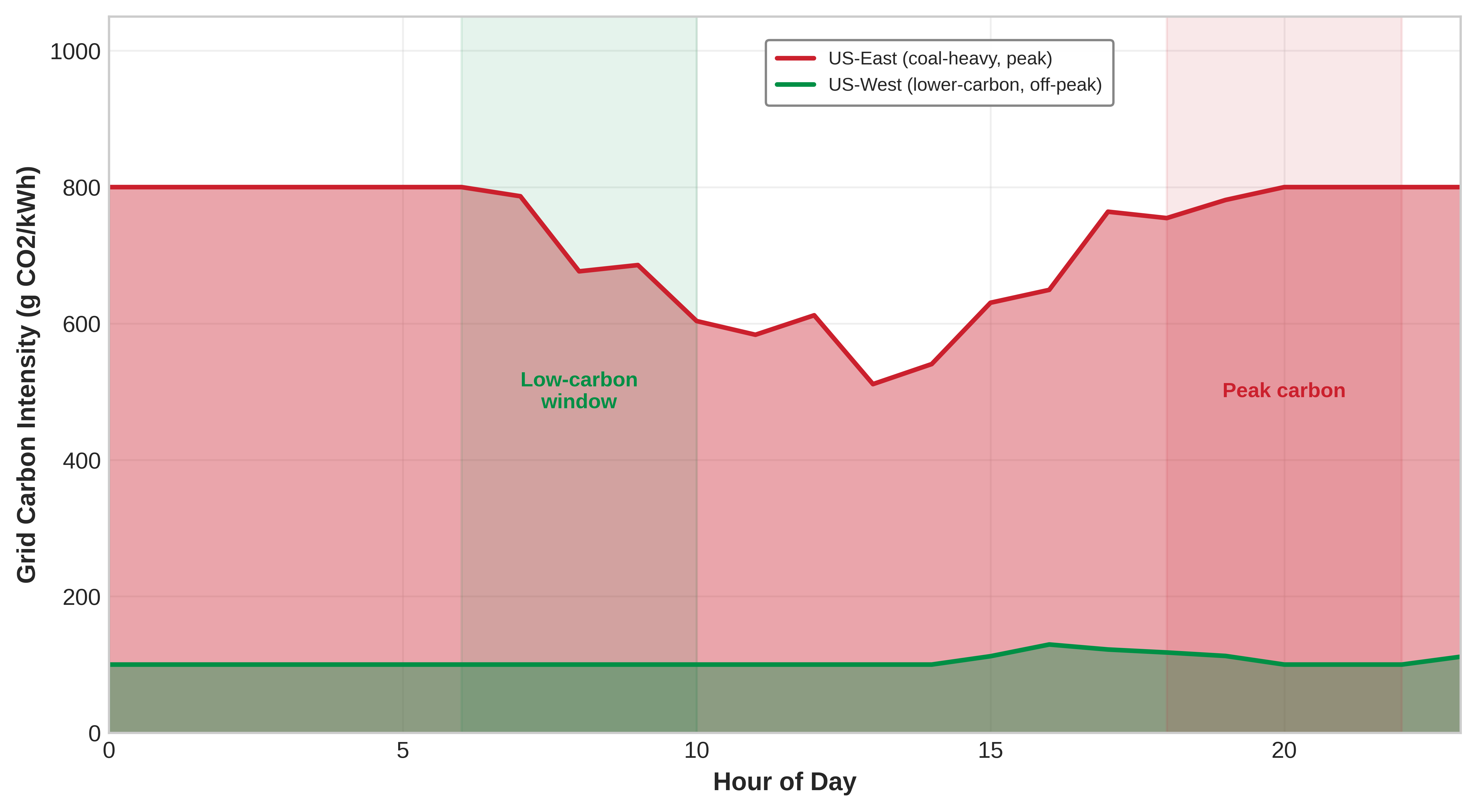
Renewable energy variability presents a key challenge for carbon-aware scheduling. Figure 24 captures European grid dynamics: solar energy peaks at midday, wind shows distinct peaks in mornings and evenings, and fossil generation fills the gaps. This temporal pattern determines when AI workloads can run on clean energy.
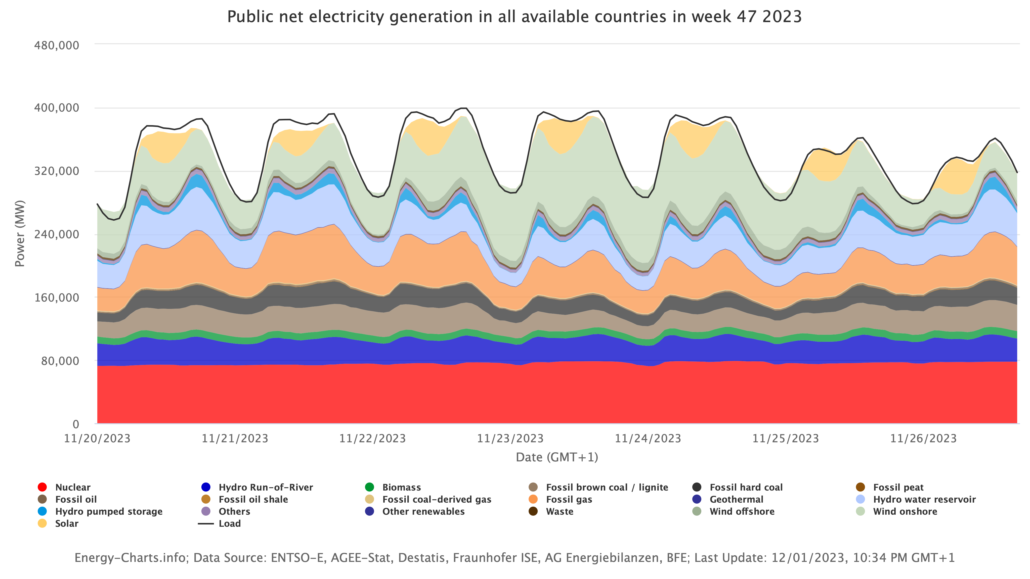
Energy-aware AI frameworks complement scheduling by optimizing the workloads themselves. Zeus (You et al. 2023) achieves 75 percent energy savings on BERT training by automatically finding optimal energy-performance trade-offs, while Perseus (Chung et al. 2023) reduces GPU memory usage by 50 percent through dynamic batching. These tools, alongside CodeCarbon for emissions tracking, democratize energy optimization beyond hyperscale companies.
You, Jie, Jae-Won Chung, and Mosharaf Chowdhury. 2023. “Zeus: Understanding and Optimizing GPU Energy Consumption of DNN Training.” 20th USENIX Symposium on Networked Systems Design and Implementation (NSDI 23), 119–39.
Chung, Jae-Won, Yile Gu, Insu Jang, Luoxi Meng, Nikhil Bansal, and Mosharaf Chowdhury. 2023. “Reducing Energy Bloat in Large Model Training.” Proceedings of the ACM SIGOPS 30th Symposium on Operating Systems Principles abs/2312.06902: 144–59. https://doi.org/10.1145/3694715.3695970.
AI-driven thermal optimization
AI-driven cooling optimization represents an immediate, software-deployable opportunity for reducing data center energy consumption. Traditional cooling systems rely on fixed control policies with predefined temperature thresholds, often consuming more energy than necessary. DeepMind’s deep reinforcement learning system continuously analyzes real-time sensor data—temperature, humidity, cooling pump speeds, and fan activity—to identify the most energy-efficient configuration for each workload. In production at Google’s data centers, this system achieved a 40 percent reduction in cooling energy usage and a 15 percent reduction in total data center power consumption.
Complementing software optimization, advances in liquid cooling and immersion cooling are transforming data center thermal management. Liquid cooling transfers heat directly from accelerator chips using specially designed coolants, achieving 3,000\(\times\) better heat transfer than air. Immersion cooling submerges entire server racks in nonconductive liquid coolants, eliminating traditional air-based systems entirely. These approaches enable higher compute densities with lower power consumption—critical as AI accelerators push thermal design power into the hundreds of watts per chip.
Case study: Google’s framework
To mitigate emissions from rapidly expanding AI workloads, Google engineers identified four key optimization areas, the “4 Ms,” where systematic improvements collectively reduce the carbon footprint of machine learning (Patterson et al. 2021):
Patterson, David, Joseph Gonzalez, Quoc Le, Chen Liang, Lluis-Miquel Munguia, Daniel Rothchild, David So, Maud Texier, and Jeff Dean. 2021. “Carbon Emissions and Large Neural Network Training.” arXiv Preprint arXiv:2104.10350.
Model: The selection of efficient AI architectures reduces computation requirements by 5–10\(\times\) without compromising model quality. Google has extensively researched sparse models and neural architecture search methodologies, resulting in efficient architectures such as the Evolved Transformer and Primer.
Machine: The implementation of AI-specific hardware offers 2–5\(\times\) improvements in performance per watt compared to general-purpose systems. Google’s TPUs demonstrate 5–13\(\times\) greater carbon efficiency relative to nonoptimized GPUs.
Mechanization: Optimized cloud computing infrastructure with high utilization rates yields 1.4–2\(\times\) energy reductions compared to conventional on-premise data centers. Google’s facilities consistently exceed industry standards for PUE.
Map: The strategic positioning of data centers in regions with low-carbon electricity supplies reduces gross emissions by 5–10\(\times\). Google maintains real-time monitoring of renewable energy usage across its global infrastructure.
The combined effect of these practices produces multiplicative efficiency gains. For instance, implementing the optimized Transformer model on TPUs in strategically located data centers reduced energy consumption by a factor of 83 and CO2 emissions by a factor of 747.
Despite substantial growth in AI deployment across Google’s product ecosystem, systematic efficiency improvements have effectively constrained energy consumption growth. A significant indicator of this progress is the observation that AI workloads have maintained a consistent 10 percent to 15 percent proportion of Google’s total energy consumption from 2019 through 2021. As AI functionality expanded across Google’s services, corresponding increases in compute cycles were offset by advancements in algorithms, specialized hardware, infrastructure design, and geographical optimization.
Empirical case studies demonstrate how engineering principles focused on sustainable AI development allow simultaneous improvements in both performance and environmental impact. For example, comparative analysis between GPT-3 (the leading model in mid-2020) and Google’s GLaM model reveals improved accuracy metrics alongside reduced training computation requirements and lower-carbon energy sources—resulting in a 14-fold reduction in CO2 emissions within an 18-month development cycle.
Google’s multifaceted strategy—combining systematic measurement, carbon-aware development, transparency in reporting, and renewable energy transition—establishes a replicable framework for sustainable AI scaling. Their analysis also revealed that previous published estimates overestimated ML’s energy requirements by 100 to 100,000\(\times\) due to methodological limitations, underscoring the importance of empirical measurement over theoretical projections.
Engineering guidelines for sustainable AI development
Measurement, optimization, and scheduling frameworks provide the analytical foundation, but implementation requires concrete, actionable steps. The following checklist consolidates practices that AI engineers can implement immediately to reduce environmental impact:
Measure First: Tools like CodeCarbon track the emissions of training runs. Teams cannot improve what they do not measure, and establishing baseline metrics is essential for validating the effectiveness of optimization efforts (Anthony et al. 2020).
Choose Region Wisely: Train models in data centers powered by renewable energy. Grid carbon intensity varies by 20–50\(\times\) across regions; scheduling workloads where clean energy is most abundant yields immediate reductions.
Optimize the Model: Avoid training the largest model possible by default. Pruning, quantization, and knowledge distillation find the smallest model that meets accuracy targets. A 90 percent accurate model requiring 10 percent of the resources often provides better real-world value than a 95 percent accurate model requiring full resources.
Avoid Retraining From Scratch: Transfer learning and fine-tuning reduce computational requirements by orders of magnitude compared to full retraining.
Select Efficient Hardware: Energy-efficient accelerators (such as TPUs or specialized inference chips) reduce deployment costs. The full hardware lifecycle and workload-specific platform selection matter as much as raw throughput.
Account for the Full Lifecycle: Longer hardware refresh cycles and responsible e-waste policies reduce total environmental impact. Manufacturing often exceeds operational energy consumption, making hardware longevity a critical sustainability factor.
Anthony, L. F. W., B. Kanding, and R. Selvan. 2020. Carbontracker: Tracking and Predicting the Carbon Footprint of Training Deep Learning Models. ICML Workshop on Challenges in Deploying and monitoring Machine Learning Systems.
The cumulative impact of individual technical choices depends on systemic, industry-wide adoption. Without external pressure, market forces prioritize speed and scale over efficiency. Policy and regulatory frameworks translate engineering possibilities into industry-wide practice by making sustainable choices a financial and legal imperative.
Self-Check: Question
A translation service halves its per-query compute after deploying distillation. Within six months, total monthly energy has risen by 40 percent because cheaper translation unlocked new product integrations — chatbots, email assistants, accessibility tools. Which concept from this section best explains the net increase, and what does it imply about efficiency-only strategies?
- Distillation reduces accuracy too much for production, so total energy rose from re-running queries — accuracy-driven rebound.
- Jevons paradox: per-unit efficiency gains lowered the effective cost of translation and triggered enough new demand that total resource consumption grew; efficiency alone cannot guarantee sustainability without usage governance.
- Carbon accounting frameworks ignore improvements below the datacenter level, so the reported rise is an artifact of incomplete measurement.
- Efficient models can only run on specialized hardware that requires manufacturing new chips, so embodied emissions explain the rise.
A team must reduce the serving footprint of a latency-sensitive 70B-parameter model on current GPU hardware. They are weighing post-training quantization, knowledge distillation, and unstructured pruning. Justify why the chapter would likely prioritize the first two before unstructured pruning.
A platform team asks which single infrastructure-layer mitigation strategy, requiring no model or code changes, offers the highest leverage for reducing emissions of an existing production workload. Which lever does the section identify?
- Carbon-aware scheduling across regions and time windows with lower grid carbon intensity, because identical workloads can differ by 20-50x in emissions purely by placement.
- Increasing batch size on every request until every workload becomes compute-bound, because higher arithmetic intensity always lowers energy.
- Replacing every deployed model with a binary neural network to cut arithmetic precision to the minimum.
- Retraining every deployed model from scratch weekly to keep it minimally sized.
When a vendor advertises a keyword-spotting accelerator’s energy-per-inference and accuracy on a microcontroller, the MLCommons benchmark suite that standardizes the tasks, measurement rules, and comparability requirements for sub-watt systems is ____.
In Google’s 4Ms sustainability framework, which element refers specifically to choosing low-carbon locations and matching workloads to cleaner electricity supply?
- Model — selecting efficient architectures.
- Machine — selecting efficient accelerators.
- Mechanization — operating cloud infrastructure efficiently.
- Map — siting and geographic workload placement to exploit regional electricity differences.
Explain why the chapter pairs technical efficiency with carbon budgets, governance, or usage limits rather than treating optimization as sufficient on its own.
Policy, Regulation, and the Path Forward
If a company can slash its cloud computing bill by relocating its training cluster to a region powered entirely by cheap, high-emission coal, the market alone will not prevent them from doing so. Engineering ingenuity can provide the tools for efficient computation, but it requires policy, regulation, and carbon pricing to ensure that using those tools becomes a financial and legal imperative rather than just a corporate public relations talking point.
Regulatory mechanisms
Effective AI sustainability governance operates through a combination of mandatory reporting, emission restrictions, and financial incentives, though global policy fragmentation presents a significant implementation challenge. The European Union has taken a leading role with mandatory approaches, notably the AI Act40 and the Corporate Sustainability Reporting Directive (CSRD).41 The AI Act creates separate obligations for general-purpose AI models and for general-purpose AI models with systemic risk, including documentation of computational resources and known or estimated model energy consumption. The CSRD mandates that large companies disclose their environmental impacts, including Scope 1, 2, and 3 emissions from AI operations, according to standardized, audited reporting frameworks. This regulatory shift transforms energy monitoring from an optional optimization into a legal necessity.
40 EU AI Act (2024): The world’s first comprehensive AI regulation creates obligations for general-purpose AI models and additional obligations for models with systemic risk, including models presumed to have high-impact capabilities above \(10^{25}\) FLOPs of training compute. Technical documentation must include computational resources and known or estimated model energy consumption. For violations by providers of general-purpose AI models, Article 101 permits fines up to 3 percent of annual worldwide turnover or EUR 15 million; the separate 7 percent maximum applies to prohibited-practice violations.
41 CSRD (Corporate Sustainability Reporting Directive): Effective 2024, this EU regulation requires 50,000+ companies to disclose audited Scope 1, 2, and 3 emissions using standardized ESRS frameworks. For AI infrastructure, CSRD forces disclosure of previously hidden costs: the embodied carbon of GPU procurement, energy from outsourced cloud training, and end-of-life hardware disposal that collectively constitute the majority of an AI system’s Scope 3 footprint.
42 Emissions Trading for Compute: The EU ETS (2005) pioneered cap-and-trade for industrial emissions; applying this model to AI compute would set aggregate energy budgets for training clusters and let organizations trade surplus capacity. The mechanism converts sustainability from a voluntary optimization into a priced constraint: organizations that invest in efficiency can sell unused allocation to less efficient competitors, creating a financial incentive aligned with the iron law’s utilization term (\(\eta\)).
Beyond measurement mandates, governments are exploring direct restriction mechanisms. These include setting limits on computational power available for training large AI models, mirroring Emissions Trading Systems (ETS)42 used in environmental policy. Such “cap-and-trade” systems for compute would force organizations to operate within predefined energy budgets or procure additional capacity, creating a market for computational carbon credits. The expansion of carbon pricing and Carbon Border Adjustment Mechanisms (CBAM) is converting the geographic location of compute into a direct financial variable—the carbon intensity of regional electricity grids can vary by over 40\(\times\), making carbon-aware scheduling a key compliance strategy.
To balance these restrictions, government incentives play a proactive role. Financial support, tax benefits, and grants for Green AI research can make sustainability a competitive advantage. Spain has committed €300 million to AI projects focused on sustainability. Governments can also use their public procurement power, mandating that vendors meet sustainability benchmarks such as operating on carbon-neutral data centers or using energy-efficient models. Broader corporate reporting frameworks—the Greenhouse Gas Protocol, TCFD, and ISSB—are increasingly scrutinizing Scope 3 emissions, encompassing the substantial embodied carbon of GPU procurement and data center construction alongside operational emissions of outsourced cloud compute.
Industry self-regulation and standards
Alongside government mandates, the AI industry is driving significant environmental improvements through self-regulation and common standards. The most visible commitments from major cloud providers—Google, Microsoft, and Amazon—focus on matching data center electricity consumption with renewable energy procurement and increasing direct clean-energy supply. Going further, the push for 24/7 Carbon-Free Energy (CFE) aims to match every hour of energy consumption with real-time clean energy procurement, moving beyond annual averages and carbon offsets that can obscure actual emissions from fossil-fuel-reliant grids (Monyei and Jenkins 2018).
Monyei, C. G., and Kirsten E. H. Jenkins. 2018. “Electrons Have No Identity: Setting Right Misrepresentations in Google and Apple’s Clean Energy Purchasing.” Energy Research &Amp; Social Science 46: 48–51. https://doi.org/10.1016/j.erss.2018.06.015.
Internal carbon pricing is another effective self-regulatory tool. By assigning a “shadow price” to carbon emissions, companies integrate environmental costs directly into financial decision-making for AI projects, naturally prioritizing investments in energy-efficient hardware and low-emission models. Voluntary checklists and open-source tools further promote accountability: the AI Sustainability Coalition and projects like CodeCarbon and ML CO2 Impact provide frameworks that allow developers to estimate and track model carbon footprints directly within their workflows.
Standardized benchmarks provide the objective data needed to validate these efforts. MLCommons, through its MLPerf benchmark suite, has incorporated power measurement protocols for both data center and edge deployments. By establishing metrics like “samples per Joule” and “Joules per token,” MLCommons enables fair, transparent comparison of AI system efficiency across different hardware and software platforms. These benchmarks, combined with independent sustainability audits from organizations like the Green Software Foundation, create a measurable mechanism for holding the industry accountable and driving competition toward genuinely greener AI.
Public engagement and environmental justice
Effective AI sustainability governance requires public support, which depends on transparency, clear communication, and equitable access. Currently, public understanding of AI’s environmental impact is limited and often polarized between narratives of technological salvation and ecological disaster. Fostering informed discourse requires moving beyond greenwashing43—the practice of making misleading claims about environmental responsibility—toward genuine, verifiable transparency.
43 Greenwashing in AI: Manifests as claiming “carbon neutrality” through offsets while expanding data center capacity, or highlighting per-query efficiency gains while total compute grows 10\(\times\). Emerging green-claims rules increasingly require verifiable evidence for environmental claims. For ML engineers, the technical litmus test is whether sustainability reporting covers all three GHG Protocol scopes, or conveniently omits Scope 3 (hardware manufacturing, cloud supply chain) where much of AI’s carbon can reside.
The Montréal Carbon Pledge offers a model for such transparency. Originally for institutional investors, its core commitment—to measure and disclose carbon footprints annually—is directly applicable to the AI industry.
“Measuring our carbon footprint is integral to understanding better, quantifying, and managing the carbon and climate change-related impacts, risks, and opportunities in our investments. Therefore, as a first step, we commit to measuring and disclosing the carbon footprint…annually.”—Montréal Carbon Pledge
Adopting a similar pledge would help build public trust by substantiating sustainability claims with data. Building public participation through citizen science, open data platforms, and inclusive governance forums ensures that AI development aligns with societal values and that its benefits are shared broadly.
The principles of environmental justice must be central to AI sustainability. The environmental burdens of AI—from resource extraction for hardware manufacturing to the siting of energy-intensive data centers—are often borne by marginalized communities, while economic benefits concentrate elsewhere. The digital divide means that access to AI-driven sustainability tools is unevenly distributed, potentially widening global inequalities. Ensuring equitable access to AI technologies, investing in capacity-building in developing nations, and requiring social impact assessments for large-scale AI projects are critical steps to ensure that the transition to a sustainable AI ecosystem is also a just one.
Future research directions
While policy and public engagement shape the context for sustainable AI, its future ultimately depends on continued technical innovation. One of the most promising areas is the development of non-von Neumann computing architectures44, such as neuromorphic computing and in-memory computing. By processing data where it is stored, these paradigms aim to eliminate the “von Neumann bottleneck”—the energy-intensive shuttling of data between memory and processing units that can account for 60–80 percent of a system’s power consumption. Successful implementation could yield energy efficiency improvements of 100–1000\(\times\) for certain AI workloads.
44 Von Neumann Bottleneck: John von Neumann’s 1945 stored-program architecture separates processing from memory, requiring constant data shuttling that consumes 60–80 percent of system power. For AI workloads dominated by matrix multiplications with low arithmetic intensity, this bottleneck means most energy moves data rather than computes results. In-memory and neuromorphic architectures attack this directly, with potential 100–1,000\(\times\) energy reductions for inference by eliminating the memory-processor round trip.
Siddik, Md Abu Bakar, Arman Shehabi, and Landon Marston. 2021. “The Environmental Footprint of Data Centers in the United States.” Environmental Research Letters 16 (6): 064017. https://doi.org/10.1088/1748-9326/abfba1.
A critical implementation barrier is the “measurement gap”: the lack of standardized, hardware-level tools for accurately measuring the environmental footprint of AI systems (Siddik et al. 2021). Current methods often rely on coarse proxy metrics—GPU-hours multiplied by average grid intensity—which fail to capture the real-world dynamics required by emerging regulations. Developing and standardizing granular, real-time energy and carbon accounting tools is essential for both compliance and effective optimization.
Furthermore, an integrated, data-centric approach is needed to minimize redundant computation. Research shows that the predictive value of training data often decays, meaning models are frequently trained on vast datasets with diminishing returns (Wu et al. 2022). Smarter data sampling, active learning, and data valuation techniques can optimize training processes to use only the most informative data, reducing computational waste without sacrificing accuracy. Ultimately, an integrated approach combining algorithmic efficiency, hardware innovation, renewable energy adoption, and transparent governance is necessary to ensure AI’s trajectory aligns with global sustainability goals.
Wu, Carole-Jean, Ramya Raghavendra, Udit Gupta, Bilge Acun, Newsha Ardalani, Kiwan Maeng, Gloria Chang, et al. 2022. “Sustainable AI: Environmental Implications, Challenges and Opportunities.” Proceedings of Machine Learning and Systems 4: 795–813.
Minimizing redundant computation through smarter data curation directly aligns regulatory compliance with operational efficiency. The most dangerous obstacles to sustainable AI are not technical limitations but incorrect assumptions—miscalculations that cause well-intentioned teams to inadvertently increase their environmental footprint.
Self-Check: Question
A sustainability team argues that carbon pricing is unnecessary because ‘rational firms will naturally choose greener options once they see the accounting.’ Which rebuttal from the section best explains why market incentives alone are insufficient?
- Datacenter operators are legally prohibited from choosing lower-cost electricity sources, so carbon choices are pre-decided by regulation.
- Without carbon pricing, the cheapest operational choice is often the dirtiest one, so firms optimizing cost will rationally pick fossil-heavy regions or hours and increase emissions even while reporting accurately.
- Renewable-powered regions always have the highest electricity prices, making green choices impossible.
- Cloud providers already disclose Scope 3 emissions with perfect accuracy, so no further mechanism is needed.
A compliance team is translating the EU AI Act and the Corporate Sustainability Reporting Directive (CSRD) into engineering requirements. Which framing best matches how the section describes their practical effect?
- Energy reporting and emissions accounting become mandatory design constraints: systems must be instrumented to produce audited Scope 1/2/3 disclosures, shifting sustainability from optional metric to compliance requirement.
- They ban foundation-model training above a fixed FLOP threshold worldwide, so the engineering question is simply whether training fits under the cap.
- They replace direct power measurement with legal estimates based only on parameter count, so no new instrumentation is needed.
- They apply only to hardware manufacturers, not to organizations operating AI services.
Explain how an emissions-trading scheme or carbon price transforms carbon-aware scheduling from a purely voluntary practice into an economically rational default.
True or False: A company purchases enough annual Renewable Energy Certificates to match 100 percent of its yearly AI electricity use, but its evening serving load runs on a grid that is 60 percent coal-fired between 6 PM and midnight. By the section’s standard, this is equivalent to meeting 24/7 clean-energy matching.
Which future research direction does the section frame as directly attacking the von Neumann bottleneck’s energy cost rather than its measurement?
- Broader adoption of annual sustainability reports so more organizations see their numbers.
- Non-von-Neumann approaches such as neuromorphic and in-memory computing that reduce or eliminate data shuttling between memory and compute.
- Increasing model size so arithmetic intensity always sits right of the memory crossover.
- Replacing lifecycle accounting with benchmark-only reporting to simplify comparison.
Fallacies and Pitfalls
Sustainability involves counterintuitive physics where efficiency improvements can increase total consumption and geographic choices dominate all other optimizations. These fallacies and pitfalls capture errors that waste compute budgets and planetary resources through misallocated optimization effort.
Fallacy: Cloud computing automatically makes AI systems more environmentally sustainable.
Engineers assume cloud providers operate efficiently and sustainably. In production, geographic region dominates all other factors through grid carbon intensity differences. Training a 7B model on 64 A100s for 14 days produces 4.4 metric tons CO2 on the US average grid (429 g/kWh) but only 206 kg CO2 on Quebec’s hydroelectric grid (20 g/kWh operational)—a roughly 21-fold difference for identical workloads, consistent with the 4,400 kg vs. 206 kg figures. Coal-powered grids emit 800–1000 g CO2/kWh while well-managed hydroelectric sources emit 10–50 g CO2/kWh. As demonstrated in Section 1.3, teams that deploy to default cloud regions without checking grid carbon intensity waste 20–50\(\times\) more carbon budget than necessary, turning “cloud sustainability” into a geographic lottery rather than an inherent advantage.
Pitfall: Focusing only on operational energy consumption while ignoring embodied carbon and lifecycle impacts.
Teams optimize training efficiency while ignoring manufacturing emissions. In low-carbon grids, embodied carbon can dominate fleet-level footprint accounting. As quantified in Section 1.3.1.1, an A100 accelerator embodies roughly 150 kg CO2 from manufacturing (Luccioni et al. 2023); for the 14-day, 64-A100 training run above, the unamortized upfront burden is roughly 9.6 metric tons CO2. Amortized over a 4-year service life, the share attributable to this specific 14-day job is about 90 kg, but the unamortized fleet-level number is what dominates total footprint accounting: it exceeds the job’s operational emissions on Quebec’s clean grid where operational emissions are minimal. Extending hardware lifetime from 3 to 5 years reduces amortized embodied carbon by 40 percent. Organizations focusing exclusively on operational efficiency miss this procurement and depreciation lever while optimizing marginal gains in PUE or compute efficiency.
Luccioni, Alexandra Sasha, Sylvain Viguier, and Anne-Laure Ligozat. 2023. “Estimating the Carbon Footprint of BLOOM, a 176B Parameter Language Model.” Journal of Machine Learning Research 24 (253): 1–15.
Fallacy: Efficiency improvements automatically reduce total environmental impact.
Engineers assume that halving inference cost cuts environmental impact in half. In production, Jevons Paradox establishes that efficiency improvements increase total consumption by enabling expanded usage. GPT-3’s launch at $0.06 per 1,000 tokens enabled applications impossible at GPT-2’s economics; reducing costs to $0.002 per 1,000 tokens (30\(\times\) improvement) triggered a 100\(\times\) increase in query volume, growing total emissions despite per-query efficiency gains. Quantization that reduces inference energy by 4\(\times\) often leads to 10\(\times\) deployment expansion as cost constraints relax. Organizations that optimize efficiency without usage governance consistently experience 3–5\(\times\) consumption growth within six months of deployment, transforming sustainability wins into consumption explosions requiring carbon budgets and usage caps of the kind motivated by the Jevons analysis in Figure 21.
Pitfall: Treating carbon offsets as a substitute for reducing actual emissions.
Organizations purchase offsets to neutralize emissions without validating offset quality. In reality, analysis of voluntary carbon markets reveals that 60–90 percent of credits fail to deliver claimed reductions due to inflated baselines, nonpermanent sequestration, or projects that would have occurred regardless. A company training models on coal grids (1000 g CO2/kWh) and buying offsets spends 2–3\(\times\) more than directly migrating to renewable regions (20–50 g CO2/kWh) while achieving inferior environmental outcomes. Offset projects take 5-20 years to sequester carbon while compute emissions are immediate. Teams that prioritize offsets over actual reduction miss the 20–50\(\times\) leverage available through geographic optimization shown in Section 1.3 and delay renewable energy transitions that deliver permanent improvements.
Pitfall: Optimizing individual components without analyzing system-level lifecycle impacts.
Teams reduce training cost to improve sustainability without analyzing deployment scale. In production, training-inference trade-offs often invert total emissions. A model pruned by 40 percent to save training energy but requiring 2\(\times\) inference compute increases total lifecycle emissions if it serves more than 100 million queries—a crossover point reached in 3-6 months for production systems. Edge deployment that reduces data center energy by 60 percent but requires manufacturing 10,000 specialized devices adds 1,500-2,000 kg embodied carbon (10\(\times\) the cloud training emissions). Extending GPU lifetime from 3 to 5 years reduces amortized embodied carbon by 40 percent but may sacrifice 15–25 percent operational efficiency; the lifecycle break-even depends on grid carbon intensity, with lifetime extension dominating on clean grids and efficiency winning on dirty grids. Effective sustainability requires holistic analysis across Section 1.3.1.2 rather than local optimization.
A model aggressively pruned to save training energy, only to require massive computational overhead during inference to compensate for lost accuracy, perfectly illustrates the danger of localized optimization. Avoiding these systemic pitfalls allows us to view the ML lifecycle holistically, bringing us to a final synthesis of sustainable AI architecture.
Self-Check: Question
True or False: A team migrates a batch-training workload from an on-premises cluster in Virginia (roughly 400 gCO2/kWh) to a cloud region in West Virginia (roughly 700 gCO2/kWh) because the cloud provider markets its AI infrastructure as ‘green.’ The migration necessarily improves the run’s carbon footprint.
A team prunes a model aggressively to cut training energy, but the resulting deployment requires custom sparse-execution hardware and more total serving compute to hit accuracy targets. Which pitfall does this scenario illustrate, and what mitigation does the section recommend?
- Higher GPU utilization always increases embodied carbon per query, so any pruning gain is automatically lost to hardware.
- Local optimization of one lifecycle component (training energy) without accounting for inference scale, manufacturing burden, and hardware support can worsen total lifecycle emissions; the mitigation is full-lifecycle accounting before committing to the optimization.
- Measuring carbon intensity too often instead of using annual averages creates an appearance of higher emissions that disappears with averaging.
- Transfer learning makes lifecycle accounting impossible because the original training is hidden upstream.
Explain why the section treats buying carbon offsets as a weaker sustainability strategy than directly reducing emissions through location or system-design decisions.
Summary
Sustainable AI represents the “physical limit” of the Machine Learning Fleet. The preceding chapters optimized the logic, constructed the hardware, launched global services, and hardened the perimeter. The final gating constraint remains the question of whether these systems can exist within the energy, water, and material boundaries of the planet.
Sustainability is a core engineering requirement, not a discretionary “nice-to-have.” The lifecycle carbon footprint spans from the 164 kg of CO2 embodied in a single H100 GPU (per NVIDIA’s product carbon footprint) to the thousands of megawatt-hours consumed during training. The “Mobile memory wall” and the “Decode Energy Problem” explain why the shift to specialized accelerators is a survival strategy for both the cloud and the edge. The “Rebound Effect” completes the picture: efficiency alone cannot solve the crisis if it leads to exponential increases in usage.
Key Takeaways: Efficiency alone is not enough
- The sustainability paradox: In the historical 2012–2019 scaling window, AI compute demand grew about 6.2\(\times\) per year, roughly 4\(\times\) faster than the 1.5\(\times\) annual hardware-efficiency curve used in this chapter. Without algorithmic intervention (for example, pruning, quantization), the Machine Learning Fleet will hit a “power wall” that constrains all future innovation.
- The inefficiency of decode: Autoregressive token generation is notoriously energy-wasteful. While prefill is compute-bound and efficient, decode is bandwidth-bound, leaving GPUs idling and drawing massive static power. Specialized, memory-optimized NPUs/TPUs are essential for sustainable serving.
- Embodied carbon is real: Up to 30 percent of a system’s lifecycle emissions occur before it is ever powered on. The manufacturing of sub-5nm chips is water- and chemical-intensive, making hardware longevity and circular economy reuse critical MLOps concerns.
- Jevons paradox: Improving the efficiency of AI tokens reduces their cost, which often triggers a massive increase in total demand. Sustainable AI requires a dual strategy: technical optimization combined with carbon-aware governance.
- Carbon-aware scheduling: Geographic placement is the highest-leverage sustainability choice. Moving a training job from a coal-powered grid to a hydro-powered one can reduce emissions by 20–50\(\times\) without changing a single line of code.
Sustainability is an engineering discipline, not a public relations exercise. Carbon budgets, power delivery constraints, and cooling capacity impose hard limits on fleet expansion that no amount of marketing language can circumvent. The Jevons Paradox makes this especially clear: efficiency gains that reduce per-query cost routinely trigger demand explosions that overwhelm the original savings, meaning that technical optimization without governance is self-defeating. Organizations that treat sustainability as a solved problem after adopting a few efficiency techniques are repeating the same mistake that drove industrial energy consumption upward for two centuries.
The practitioner who can quantify lifecycle carbon across training, inference, and embodied manufacturing emissions, and who can design carbon-aware scheduling policies that respect grid carbon intensity, is increasingly essential to production ML teams. These skills transform sustainability from an abstract corporate goal into a measurable engineering constraint with the same rigor applied to latency budgets or memory capacity. As regulatory frameworks mature and carbon pricing mechanisms expand, the ability to account for and minimize environmental impact will become as fundamental to ML systems engineering as fault tolerance or security.
What’s Next: From sustainability to responsibility
The environmental footprint of the ML fleet is now quantified and constrained, ensuring that systems remain viable as they scale. Security, robustness, and sustainability together form the engineering foundation of production AI. A system that is technically sound, however, can still cause social harm.
In Responsible Engineering, we turn to the governance frameworks, fairness requirements, and ethical guardrails that ensure our fleet serves the values of the society that built it, completing the transition from how to build the machine to whom it serves.
Self-Check: Question
Which statement best captures the chapter’s overall sustainability thesis?
- Sustainability is primarily an infrastructure sourcing problem: once per-query model efficiency is good enough, only the procurement team’s choice of renewable providers matters.
- Sustainability is a physical systems constraint on energy, cooling, carbon, water, and materials that can determine whether an ML system is deployable at all, and it must be reasoned about at every layer from architecture to governance.
- Sustainability is equivalent to running workloads on renewable power and can be separated from hardware design and inference engineering.
- Sustainability matters mainly for training because inference and hardware manufacturing are comparatively small contributors to total impact.
Explain why the chapter’s final message ties decode inefficiency, embodied carbon, and Jevons paradox into a single argument rather than treating them as separate issues.
A production team needs the highest immediate emissions reduction without changing model code. Which intervention does the chapter’s synthesis identify as the single highest-leverage near-term lever?
- Increasing parameter count to improve output quality so fewer retries are needed per user session.
- Moving the workload from a coal-heavy grid to a low-carbon region through carbon-aware scheduling, since identical workloads can differ by 20 to 50x in emissions purely by placement.
- Dropping facility PUE through a cooling-upgrade program, accepting a 12-to-18-month capital project to realize a roughly 5-10 percent reduction in total facility energy.
- Applying post-training quantization to the deployed model to cut serving energy by a single-digit percentage per query.
Self-Check Answers
Self-Check: Answer
A hyperscaler commits to a 500 MW campus for a new training cluster, but the local grid interconnect approval is capped at 320 MW for the next three years. The company’s credit line would cover the projected electricity bill five times over. Which framing best captures why the chapter treats sustainability as a first-class engineering constraint rather than a reporting concern?
- Carbon accounting rules require disclosing the full planned capacity before any portion can be energized, so the 180 MW gap creates a compliance problem the team must file before training begins.
- Power-delivery and grid-interconnect capacity impose a physical ceiling that dollars cannot resolve on the required timescale, so the 180 MW gap becomes an infeasibility the training plan must route around.
- Electricity price volatility makes the 180 MW gap a budgeting risk, so the primary response is to hedge power contracts and continue the original training plan.
- Public concern about AI ethics will force the company to match every unapproved megawatt with offsets, adding cost but not changing what can be built.
Answer: The correct answer is B. The chapter’s thesis is that sustainability is a physical ceiling, not a reporting or accounting artifact: a 500 MW plan against a 320 MW approved interconnect cannot be solved by paying more per kWh. An accounting-focused framing misses that the binding constraint is kilowatts delivered, not dollars spent; a pricing-hedge framing treats capacity as a cost problem rather than an availability problem.
Learning Objective: Classify the binding constraint in a capacity-limited training deployment and justify why energy is a physical rather than financial concern
A team plans a 10,000 MWh training run. Their procurement team can route it to Quebec at roughly 20 gCO2/kWh or Poland at roughly 800 gCO2/kWh, or invest six engineer-months in a 15 percent algorithmic speedup that runs at the Poland site. Using the section’s carbon-intensity reasoning, justify which lever the team should pull first and quantify the difference.
Answer: Geographic placement multiplies the same 10,000 MWh by the grid’s gCO2/kWh factor, so the Quebec run emits roughly 200 tonnes CO2 while the Poland run emits roughly 8,000 tonnes — about 40x. A 15 percent compute reduction in Poland only cuts the 8,000 tonnes to about 6,800 tonnes, still more than 30x the Quebec footprint. The practical implication is that grid selection dominates modest algorithmic gains: the team should schedule in Quebec first and treat the algorithmic speedup as a complementary, not substitute, optimization.
Learning Objective: Analyze why grid carbon intensity typically dominates single-digit-percent algorithmic improvements in training-scale workloads
True or False: Because specialized accelerators have delivered order-of-magnitude energy-efficiency gains each hardware generation, a team can plan a decade-long AI strategy that relies on continued silicon improvements alone to keep total datacenter power flat.
Answer: False. The section shows AI compute demand has grown far faster than per-operation efficiency gains — roughly 6.2 times per year against a few times per generation — so silicon improvements are swamped by model-scale growth. A plan that counts on hardware alone ignores the demand curve that actually sets total draw.
Learning Objective: Evaluate the claim that hardware efficiency gains alone can offset exponential AI compute demand growth
Order the following events during a synchronized gradient-update step in a large training cluster when they create a grid-side transient: (1) GPUs resume a compute phase and cluster draw returns toward peak, (2) on-site batteries or supercapacitors absorb the dip and smooth the voltage, (3) thousands of GPUs simultaneously pause for AllReduce, causing a sudden drop in cluster power draw.
Answer: The correct order is: (3) thousands of GPUs simultaneously pause for AllReduce, causing a sudden drop in cluster power draw, (2) on-site batteries or supercapacitors absorb the dip and smooth the voltage, (1) GPUs resume a compute phase and cluster draw returns toward peak. The synchronization pause must precede the buffering, because the buffer exists to smooth a transient it can only respond to; and the compute phase resumes after the buffer has released the stored energy. Swapping pause and buffering would imply the mitigation fires before any disturbance exists — and swapping buffering and resume would strand the grid through a second, unabsorbed swing.
Learning Objective: Sequence the causal chain from synchronized compute pauses to on-site buffering in distributed training, and identify what breaks if steps are reordered
A research group wants to cut AI energy use without assuming the grid will keep scaling. Which architectural direction most directly attacks the root cause of the inefficiency the section identifies?
- Keeping every layer and attention head active on every input so utilization is always high, because higher utilization always means better efficiency.
- Event-driven and sparse-activation architectures that compute only on changes or salient inputs, because most of today’s energy pays for dense, globally synchronized data movement.
- Replacing all ReLU activations with a different pointwise nonlinearity to shave a small fraction of arithmetic per layer.
- Deferring sustainability work until emissions reporting standards stabilize, because architectural choices cannot be justified without fixed metrics.
Answer: The correct answer is B. The section argues the energy wall comes from dense, globally synchronized computation and the data movement it forces, so event-driven and sparse-activation designs target the physical root cause. An always-on framing conflates utilization with efficiency — hardware kept busy on unnecessary work burns energy without producing value. Swapping a nonlinearity trims a small constant; it does not change the data-movement regime that dominates energy.
Learning Objective: Select an architectural direction that addresses data-movement dominance in AI energy consumption
Self-Check: Answer
A profiling run on an accelerator with approximately 10 pJ per FLOP of compute energy and approximately 100 pJ per byte of DRAM energy reports an arithmetic intensity of 3 FLOPs per byte for an attention kernel. Which optimization family is most likely to move this workload closer to the energy roofline?
- Replacing the accelerator with one that advertises 2x the peak FLOPS per watt while keeping the memory subsystem unchanged, because raising the compute ceiling always lowers energy.
- Fusing operators and tiling to keep intermediate activations in on-chip SRAM, because the kernel sits far to the left of the energy crossover at about 10 FLOPs per byte and pays most of its joules in DRAM traffic.
- Prioritizing a PUE reduction on the facility because chip-level bottlenecks do not affect per-query energy.
- Raising numerical precision from FP16 to FP32, because higher precision does more useful work per byte read.
Answer: The correct answer is B. Dividing e_byte by e_flop gives a crossover near 10 FLOPs per byte; a kernel at 3 FLOPs per byte is memory-energy bound, so joules come from data movement and fusion or tiling directly reduces them. A compute-ceiling swap attacks the wrong term — the kernel is not compute-bound. PUE multiplies total energy but does not change which on-chip term dominates. Raising precision increases both FLOPs and bytes, worsening the problem.
Learning Objective: Apply the energy-roofline crossover to classify a workload’s dominant energy term and select the matching optimization family
A 2 MW cluster drops its PUE from 1.58 to 1.10 without changing any model code or hardware SKU. Explain why the chapter counts this as a first-order sustainability intervention, and quantify roughly what the facility saves per year.
Answer: Total facility power is IT load multiplied by PUE, so the 2 MW IT load shifts from 3.16 MW to 2.20 MW of total draw — a saving of about 0.96 MW, or roughly 8,400 MWh per year at 24/7 operation. The saving is realized without touching model architecture, dataset, or accelerator choice: every joule the model spends now carries less cooling and power-distribution baggage. The practical consequence is that facility engineering is on the same leverage tier as a large algorithmic optimization; infrastructure-layer work can deliver model-optimization-sized wins.
Learning Objective: Analyze how facility-level efficiency changes total AI energy consumption independent of model and hardware changes
An engineer must profile energy for a battery-powered microcontroller running a wake-word detector that sleeps most of the second. The device has no internal power counters and draws microwatts during deep sleep. Which measurement approach best matches the section’s edge methodology?
- Sample a tool such as nvidia-smi at 10 Hz and integrate the series, because server-grade sampling tools work across platforms.
- Use an external current-sense monitor such as an INA219 or Joulescope, sample at a rate that resolves the active burst and deep-sleep transitions, and explicitly account for duty cycle, warm-up, and peripherals.
- Estimate total energy by multiplying parameter count by a fixed J-per-parameter constant, because compute energy is the dominant term in TinyML.
- Rely on CPU-package RAPL counters, because they generalize from server CPUs to microcontroller-class devices.
Answer: The correct answer is B. Sub-watt edge devices lack on-chip energy counters, so external instrumentation is the only way to capture the sleep-versus-burst behavior that actually dominates average power. A parameter-count estimate ignores sleep state, peripherals, and radio activity, which typically outweigh arithmetic on duty-cycled devices. nvidia-smi and RAPL are instruments tied to data-center-class silicon; they do not exist on this platform.
Learning Objective: Select an appropriate energy-measurement method for microcontroller-class edge systems with no internal counters
A facility reports 4.2 MW of compute IT load and 6.3 MW of total site draw over the same hour. The sustainability team wants a single scalar that captures how much the non-IT infrastructure contributes to the total, so they can compare the site to peers year over year. Which metric gives them exactly that ratio, and what does a drop in it imply?
- Grid carbon intensity; a drop means the grid has decarbonized.
- Arithmetic intensity; a drop means the workload has become more memory-bound.
- PUE, computed as 6.3 / 4.2 = 1.5; a drop means every joule of useful IT work now carries less cooling and power-distribution overhead.
- Model FLOPs utilization; a drop means the accelerators are underused.
Answer: The correct answer is C. PUE is total facility power divided by IT power — here, 1.5 — and it captures exactly the non-IT overhead the team wants to track. A lower PUE means the same compute work carries less cooling and distribution energy. Grid carbon intensity describes the electricity source, not the facility’s efficiency; arithmetic intensity and MFU are workload metrics, not facility metrics.
Learning Objective: Apply the facility-efficiency metric that translates IT power into total facility power and interpret its direction of change
A profiling sweep across a training workload shows element-wise normalization and activation kernels spending roughly 8x more joules on HBM reads than on arithmetic. The service owner proposes four follow-ups. Which best matches the energy model this section develops?
- Upgrading to a newer accelerator with 2x peak tensor-core FLOPS, because more FLOPS always lowers total energy per step.
- Fusing the normalization and activation into adjacent matrix-multiply kernels so intermediate tensors stay in on-chip SRAM and round-trips to HBM collapse.
- Ignoring the kernel and investing only in carbon-aware scheduling, because chip-level energy is negligible once the grid is considered.
- Raising numerical precision to FP32 to make each byte of DRAM carry more useful arithmetic.
Answer: The correct answer is B. The section emphasizes that for low-intensity kernels, DRAM energy dominates arithmetic energy; fusion removes entire HBM round-trips by keeping intermediates in SRAM. A tensor-core upgrade raises the compute ceiling, which is the wrong lever when memory traffic is the bottleneck. Carbon-aware scheduling complements but does not replace chip-level work. Raising precision increases both FLOPs and bytes, making the kernel more memory-bound, not less.
Learning Objective: Compare the energy significance of computation and data movement and select the optimization that targets the dominant term
A team proposes to report total AI system energy as the simple sum of CPU, GPU, memory, and network component measurements. Explain why the section rejects this accounting and what form the corrected total must take.
Answer: Component measurements capture IT energy but exclude cooling, power conversion, lighting, and distribution losses that are real energy draws on the grid. The section requires multiplying IT energy by PUE so that a 1 MW IT load in a 1.4 PUE facility is accounted as 1.4 MW of total draw. The practical implication is that workload-level profiling is necessary but not sufficient; engineering and accounting decisions must tie component numbers to facility overhead to match actual grid impact and carbon reporting.
Learning Objective: Justify why facility overhead must be incorporated into total energy accounting for AI systems
Self-Check: Answer
Two engineers disagree about how to report the carbon footprint of a training run that used leased GPUs in a hydro-powered region. Which framing correctly separates operational and embodied carbon per this section’s equations?
- Operational carbon is the manufacturing and shipping footprint of the GPUs, while embodied carbon is the grid electricity used while training.
- Operational carbon is the electricity used during training and inference multiplied by grid intensity and facility PUE, while embodied carbon is the pre-use footprint of hardware and construction amortized over useful lifetime.
- Operational carbon applies only to cloud training, while embodied carbon applies only to on-premises hardware.
- Operational carbon is a concern only on fossil-heavy grids, while embodied carbon is a concern only for edge devices.
Answer: The correct answer is B. The section defines operational carbon through the E x CI x PUE product and embodied carbon as the pre-use and end-of-life footprint amortized over lifetime. A version that assigns manufacturing to ‘operational’ inverts the definitions. Tying operational to deployment model or embodied to form factor confuses where the terms apply with what the terms mean.
Learning Objective: Differentiate operational and embodied carbon and connect each to its defining equation
A team moves a training run from a fossil-heavy grid at roughly 800 gCO2/kWh to a hydro-powered grid at roughly 20 gCO2/kWh. They are surprised when their sustainability dashboard shows embodied carbon becoming the dominant term rather than operational. Explain the mechanism that causes this inversion and what it implies for hardware decisions.
Answer: Operational carbon scales linearly with grid intensity, so a 40x cleaner grid shrinks the operational term by roughly 40x while manufacturing and infrastructure emissions remain fixed per device. The embodied term, previously hidden under a large operational bar, now represents a large fraction of total footprint — the section shows it can even exceed operational on the cleanest grids. The practical consequence is that on clean grids, extending hardware refresh cycles and maximizing accelerator utilization become first-order sustainability decisions, because those are the levers that amortize the now-dominant embodied term.
Learning Objective: Analyze why grid decarbonization shifts the dominant sustainability term from operational to embodied carbon
True or False: A model trained in a datacenter powered 100 percent by hydroelectricity can honestly be reported as having a zero carbon footprint for its training run.
Answer: False. Even with zero operational emissions from hydro, the GPUs, interconnect, and facility concrete carry embodied carbon from fabrication, transport, and construction. The section shows these pre-use emissions remain and must be amortized over the run’s share of device lifetime, so total carbon is not zero.
Learning Objective: Evaluate the common fallacy that renewable electricity sourcing eliminates lifecycle carbon
A deployed model serves 10 million queries per day at 0.001 kWh per query. Its single training run consumed 1,287 MWh. Using the section’s lifecycle reasoning, what is the most important accounting consequence?
- Training still dominates because a training run uses specialized accelerators at higher per-chip peak power than serving.
- Embodied carbon can be ignored because inference energy is metered daily.
- Cumulative serving energy can exceed the one-time training energy within months — 10 million queries at 0.001 kWh is 10 MWh per day, so the 1,287 MWh training is matched in roughly 130 days — making inference efficiency the highest-impact production lever.
- The main optimization target should be compressing training time even if it raises per-query inference energy.
Answer: The correct answer is C. The arithmetic sets the cumulative inference energy on a path to cross the one-time training footprint in about four months at this query volume, so for widely deployed models, serving-side efficiency dominates. A per-step-power argument misses that cumulative volume overwhelms instantaneous power. Ignoring embodied carbon understates total footprint; accelerating training at the expense of per-query energy is precisely the wrong trade at this scale.
Learning Objective: Infer when cumulative inference energy overtakes training energy in production systems and identify the implied optimization target
Order the following steps of a lifecycle carbon estimate for a training run: (1) amortize hardware manufacturing and construction emissions over device lifetime to compute the run’s embodied share, (2) compute total facility energy from IT energy and PUE, (3) aggregate operational and embodied components into the lifecycle total, (4) convert operational energy to operational carbon by multiplying by grid carbon intensity.
Answer: The correct order is: (2) compute total facility energy from IT energy and PUE, (4) convert operational energy to operational carbon by multiplying by grid carbon intensity, (1) amortize hardware manufacturing and construction emissions over device lifetime to compute the run’s embodied share, (3) aggregate operational and embodied components into the lifecycle total. Facility energy is the input operational carbon needs; the operational-carbon conversion cannot happen before energy is known; and the embodied share is independent but must exist before the final aggregation. Aggregating earlier would sum incomplete quantities and hide which term actually dominates.
Learning Objective: Sequence the operational and embodied steps of a lifecycle carbon accounting workflow
Self-Check: Answer
A facility engineer is redesigning a datacenter aisle to host training racks after hosting web-serving racks for a decade. Which property of AI workloads most forces the redesign, relative to a typical web stack?
- AI workloads demand sub-millisecond tail latency that web stacks do not, so racks must be packed less densely to keep idle spares available.
- AI training holds large numbers of accelerators near peak utilization for weeks, creating sustained thermal density and power draw rather than the bursty CPU spikes web stacks produce.
- AI workloads use less energy per request than web traffic, so the real change is accounting rules rather than physical design.
- AI workloads avoid cooling needs because regular matrix arithmetic produces less heat than irregular web request patterns.
Answer: The correct answer is B. The section contrasts short-lived web bursts with training clusters that run hot for months, and the sustained thermal density — not any burstiness — is what forces power-delivery and cooling redesign. A tail-latency framing describes serving, not the training pattern under discussion; a regular-arithmetic-means-less-heat claim inverts the physics — regular high-FLOPS arithmetic produces more heat, not less.
Learning Objective: Compare the sustained power and thermal profile of AI training workloads to traditional web workloads
A team consolidates training jobs from a fleet at 45 percent average utilization onto a smaller active cluster at 85 percent utilization, powering down the drained nodes. Explain why this yields a sustainability win even if no model becomes more accurate, and state what part of the section’s total-energy model it targets.
Answer: At 45 percent utilization, the fleet’s fixed overhead — idle power, cooling for the whole building, embodied carbon per device — is amortized across little useful work, so energy and carbon per model trained are high. Consolidating to 85 percent lets the same useful work complete on fewer active devices while idle nodes enter low-power states, cutting both operational and embodied energy per training job. The practical implication is that scheduling and tenancy design reduce the energy bill without touching model architecture at all, attacking the denominator of energy-per-useful-work directly.
Learning Objective: Analyze how consolidation-driven utilization gains reduce energy consumed per unit of useful training work
A team doubles the number of GPUs in a distributed training job, expecting roughly linear energy scaling. Instead, they observe networking energy growing much faster than 2x. Which mechanism does the section identify as the primary cause, and what sustainability risk does it create?
- Total arithmetic decreases, so the model has to train longer to recover lost FLOPs, raising total energy.
- AllReduce and all-to-all gradient synchronization scale worse than linearly with cluster size and can add 20 to 40 percent to total energy, making naive cluster-size scaling carbon-inefficient.
- Facility PUE automatically worsens in direct proportion to node count regardless of cooling design.
- Embodied carbon per chip vanishes once a model is split across enough nodes, masking the true energy cost.
Answer: The correct answer is B. The section identifies gradient-synchronization traffic as a first-order energy term that can add 20 to 40 percent of total energy and scales super-linearly with parallelism, so doubling nodes can more than double networking energy. A PUE-scales-with-nodes claim confuses a facility metric with a parallelism tax. An embodied-carbon-disappears claim inverts the accounting — splitting the work across more chips increases total embodied exposure, not decreases it.
Learning Objective: Analyze how distributed-training communication patterns contribute to total cluster energy as parallelism scales
**You are auditing carbon accounting for a team running training on a leased GPU cluster. The team reports five emissions sources as shown. Which classification across the GHG Protocol scopes is correct?
S1: Diesel burned by backup generators the team owns on-site. S2: Electricity purchased from the grid to power the leased GPUs. S3: Cooling electricity drawn inside the same datacenter. S4: The embodied carbon from manufacturing the accelerators themselves. S5: Energy used by end-user phones that run the deployed model.**
- S1 Scope 1; S2 Scope 2; S3 Scope 2; S4 Scope 3; S5 Scope 3.
- S1 Scope 2; S2 Scope 1; S3 Scope 3; S4 Scope 3; S5 Scope 2.
- S1 Scope 3; S2 Scope 3; S3 Scope 2; S4 Scope 1; S5 Scope 1.
- S1 Scope 1; S2 Scope 1; S3 Scope 1; S4 Scope 2; S5 Scope 2.
Answer: The correct answer is the first option (S1 Scope 1, S2 Scope 2, S3 Scope 2, S4 Scope 3, S5 Scope 3). Direct on-site combustion the reporter owns — the diesel generators — is Scope 1. Purchased electricity for both GPUs and the cooling that supports them is Scope 2; the ‘cooling is Scope 3’ confusion shows up in practice but cooling drawn from the facility’s purchased-electricity meter is indirect energy use, not a value-chain flow. Embodied manufacturing and downstream device energy are classic Scope 3 value-chain items. An answer that places purchased electricity in Scope 1 misreads direct combustion vs. indirect energy; an answer placing embodied manufacturing in Scope 2 confuses purchased energy with purchased goods.
Learning Objective: Classify a mixed portfolio of emissions sources across the GHG Protocol scopes
Which example is most clearly Scope 3 in the chapter’s accounting framework rather than Scope 1 or Scope 2?
- Diesel burned by backup generators owned by the datacenter operator.
- Grid electricity purchased to power a leased GPU cluster.
- Cooling electricity consumed inside the datacenter and billed on the same meter as compute.
- Embodied carbon from manufacturing accelerators plus downstream energy used by end-user devices running the deployed service.
Answer: The correct answer is D. Scope 3 captures value-chain effects upstream and downstream of the operator — hardware manufacturing and end-user device energy fall there and are often large but undercounted. Generator diesel is direct on-site combustion (Scope 1); grid electricity for GPUs and cooling is purchased indirect energy (Scope 2). The Scope 3 breadth is why the chapter treats supply-chain and downstream use as a first-order engineering concern.
Learning Objective: Distinguish value-chain Scope 3 emissions from direct and purchased-energy scopes in AI systems
Self-Check: Answer
A model costs 1,287 MWh to train once and then serves 10 million queries per day at 0.001 kWh per query for a five-year product life. Which explanation best captures why inference often dominates lifecycle energy for widely deployed models?
- Inference always uses more power per operation than training because of serving-specific hardware.
- The model must be retrained on every query once in production, so inference and retraining overlap.
- Inference runs continuously across enormous cumulative query volume — here, about 10 MWh per day — so after roughly 130 days the cumulative serving energy matches the one-time training run, and after five years it dwarfs it.
- Inference cannot use specialized accelerators, unlike training, so it draws more grid power per step.
Answer: The correct answer is C. The chapter frames training as a concentrated burst and inference as an airline-like continuous operation; the cumulative volume, not per-step power, is what makes inference dominate. A ‘more power per operation’ framing is simplistic — per-step serving power is typically lower, not higher, than training. A ‘retrained every query’ claim describes no real production system; a ‘no accelerators for inference’ claim inverts current practice.
Learning Objective: Analyze why cumulative inference energy dominates one-time training energy for widely deployed production models
A profiler shows that the decode phase of an LLM serving stack sustains only 6 percent of peak FP16 TFLOPS while HBM bandwidth sits near 90 percent utilization and static power keeps flowing. Which mechanism does the section identify as the dominant source of decode energy inefficiency, and what does it imply for optimization?
- Decode disables on-chip caches, so all work shifts to the CPU and server-class RAM.
- Decode is memory-bandwidth-bound — each token requires reading the model’s weights while the compute units idle — so the accelerator burns static power without producing proportional useful work; the fix is to reduce bytes read through quantization, smaller KV caches, or weight fusion.
- Prefill uses lower numerical precision while decode must always use FP32, so decode pays a precision tax.
- Decode inefficiency comes from a transient rise in facility PUE during serving hours.
Answer: The correct answer is B. Autoregressive decode fetches all weights for each token and cannot batch temporal dependencies, saturating HBM while leaving compute idle — static power still flows regardless. Optimizations that shrink bytes per token (quantization, KV-cache compression, paged attention) move the workload back toward the roofline. The cache-disabling and precision claims invent mechanisms not in modern decoders; PUE is a facility metric and cannot explain a per-kernel bandwidth signature.
Learning Objective: Explain the systems mechanism behind the decode phase’s energy inefficiency and identify the optimization family that addresses it
A product manager claims that moving inference from the cloud to 50 million edge devices automatically solves the deployment’s sustainability problem. Explain why the chapter considers this claim incomplete and identify the lifecycle terms the edge decision can actually shift.
Answer: Edge deployment reduces transmission and cloud-compute energy per query, but 50 million devices aggregate non-trivially and introduce a large new embodied-carbon footprint from manufacturing and eventual disposal. The section shows fleet-scale edge can beat cloud only when device power budgets, duty cycles, and lifetime extension are all designed for — otherwise embodied emissions and e-waste can outweigh the operational savings. The practical implication is that edge is a conditional win: it shifts the dominant term from operational-cloud to embodied-device, so the design must amortize hardware over long service lives and drive per-device energy toward idle-dominated profiles.
Learning Objective: Evaluate the sustainability trade-offs of shifting inference from cloud to edge and identify which lifecycle terms the move actually shifts
A keyword-spotting sensor runs 10 ms of active inference once per second and sleeps the remaining 990 ms at microwatt draw. Active power is 120 mW; sleep power is 50 uW. Which quantity most strongly determines the device’s average power, per the section’s duty-cycle reasoning?
- The duty cycle, because 0.010 / 1.000 x 120 mW plus (0.990 / 1.000 x 0.050 mW) is roughly 1.25 mW — the active burst dominates this average, but the low duty cycle keeps power far below continuous 120 mW operation.
- The datacenter’s hourly carbon intensity, because the sensor uploads to a cloud pipeline.
- The model’s total parameter count, because larger models always consume more per-second energy.
- Whether the model was distilled from a larger teacher, because distillation changes average power directly.
Answer: The correct answer is A. The arithmetic gives 1.2 mW from the active window plus 0.05 mW from the sleep window, or roughly 1.25 mW total. For these values the active burst dominates the average, but the 1 percent duty cycle keeps average draw orders of magnitude below continuous 120 mW operation. Grid intensity is irrelevant to a battery-powered sensor’s own draw. Parameter count and distillation shape active power but do not change the duty-cycle arithmetic.
Learning Objective: Apply duty-cycle arithmetic to estimate average power in TinyML deployments and identify which term dominates
A startup wants to support nightly on-device full fine-tuning of a 1B-parameter model on consumer smartphones. Explain why the chapter argues this is infeasible within a realistic overnight battery budget and which class of methods it recommends instead.
Answer: Backpropagation through a 1B-parameter model requires storing activations for the full backward pass and performing roughly three times the compute of a forward pass, which on a phone with a 15 Wh battery exhausts a 5 percent overnight budget within minutes — far short of the weight updates the team wants. The section argues this is the battery wall: the energy budget is fixed by battery chemistry, not by model engineering. The recommended direction is PEFT — low-rank adapters or sparse updates — which modify only a small fraction of parameters and avoid storing full-model activations, fitting within a realistic overnight share of the battery.
Learning Objective: Justify why full backpropagation is energy-infeasible for large on-device models and identify the PEFT-family solution
Order the following stages in a hierarchical wake-word cascade designed to minimize average power on a battery-powered smart speaker: (1) full large-model inference on the captured utterance, (2) ultra-low-power voice-activity detection running continuously at microwatts, (3) small neural wake-word detector running only when voice is present.
Answer: The correct order is: (2) ultra-low-power voice-activity detection running continuously at microwatts, (3) small neural wake-word detector running only when voice is present, (1) full large-model inference on the captured utterance. The cascade must filter cheaply before escalating: the microwatt voice detector runs always, the small wake detector fires only when voice is present, and the full model fires only on a confirmed wake — each stage gating the next. Swapping the full model to the front defeats the cascade, since it would burn hundreds of milliwatts on every ambient noise event.
Learning Objective: Sequence the stages of a hierarchical wake-word cascade and justify why the ordering is necessary for sub-milliwatt average power
Self-Check: Answer
A procurement team is deciding whether to extend accelerator lifetime from three to five years. Which argument from this section best justifies treating the extension as one of the highest-leverage sustainability interventions?
- Older accelerators always become more energy-efficient after firmware updates, so per-query energy falls.
- Manufacturing emissions are large enough that amortizing them over five years instead of three cuts embodied carbon per year by roughly 40 percent, often yielding larger reductions than many per-query algorithmic optimizations.
- Datacenter PUE automatically improves as hardware ages because older chips accept higher inlet temperatures.
- Extending lifetime eliminates the need for recycling infrastructure because nothing ever leaves service.
Answer: The correct answer is B. Embodied carbon is amortized over useful life, so stretching that life from three to five years reduces the per-year share by roughly 40 percent without any runtime change. A firmware-makes-hardware-more-efficient framing confuses amortization with performance-per-watt. A PUE-improves-with-age claim inverts facility physics. An elimination-of-recycling claim ignores that all hardware eventually reaches end of life.
Learning Objective: Justify hardware lifespan extension as a high-leverage sustainability intervention
A paper reports that training a model consumed 480 MWh for its final run. Explain why this number systematically understates the development phase’s environmental impact and name the mitigation categories the chapter recommends.
Answer: The reported number covers only the final successful run, not the hyperparameter sweeps, architecture searches, debug restarts, and abandoned experiments that preceded it — and those can add an order of magnitude on top, as early neural architecture search work showed with 43,000-plus GPU-hour budgets. The mitigation categories are transfer learning to avoid training from scratch, more efficient search methods such as evolutionary or gradient-based NAS, and experimental discipline such as early stopping and shared ablation baselines. The practical implication is that sustainability accounting must capture the full research loop, not the triumphal final number.
Learning Objective: Analyze why experimentation overhead must be included in sustainability assessment of model development
True or False: A hyperscaler migrates all training workloads to a 100 percent hydro-powered region. Because operational carbon per training run is now near zero, the use phase is no longer a meaningful engineering concern — only manufacturing emissions remain.
Answer: False. A clean grid zeroes the operational carbon term but does not eliminate use-phase constraints: 24/7 inflexible load, cooling overhead, renewable timing mismatches, and grid dynamics such as the duck curve still shape what the facility can actually run when. Clean electricity changes the carbon mix; it does not remove the operational systems problem.
Learning Objective: Evaluate how a cleaner grid changes, but does not eliminate, use-phase operational constraints
A consumer-electronics company plans to ship 200 million embedded-AI sensors over five years, each with a 2-year expected lifetime and a sealed non-serviceable enclosure. Which disposal-phase concern does the section emphasize most for this product class?
- Their per-device carbon footprint is negligible because each draws only microwatts, so aggregate e-waste can be ignored.
- They will be easy to recycle because standardized components and modular batteries enable automated recovery.
- Their combination of short lifetimes, sealed enclosures, non-replaceable batteries, and enormous scale creates a distributed e-waste stream that is hard to recover, refurbish, or safely dispose of.
- They matter primarily because their on-device models drift faster than cloud models.
Answer: The correct answer is C. The section highlights short lifetimes, sealed enclosures, non-replaceable batteries, and massive scale as the defining embedded-AI e-waste problem. A low-per-device-power argument conflates operational energy with disposal impact — lifecycle accounting does not stop at the watt-hour. A standardized-components claim inverts the current reality, where embedded devices are typically less, not more, modular than servers. Model drift is a software concern, not a lifecycle-disposal concern.
Learning Objective: Identify the primary lifecycle risk introduced by large-scale embedded AI deployment
A company is considering replacing its entire accelerator fleet because the new generation offers an 8 percent improvement in performance per watt. Which response best matches the section’s circular-economy logic?
- Refresh immediately, because any efficiency gain automatically outweighs manufacturing emissions.
- Retire the old fleet the moment peak benchmark performance falls below the new generation, even if the old hardware still serves lower-priority workloads well.
- Keep the older systems in secondary roles such as batch inference, development, or non-SLA internal workloads, and upgrade only components where modular upgrades are possible, because avoiding premature disposal often beats single-digit-percent runtime gains.
- Seal the existing hardware stack more tightly so maintenance costs fall even if repair becomes impossible.
Answer: The correct answer is C. The circular-economy argument is that embodied carbon dominates small per-watt gains at single-digit percentages; keeping hardware in service via secondary deployment and modular upgrades amortizes the existing embodied cost while avoiding new manufacturing. The ‘any gain automatically justifies replacement’ framing ignores the manufacturing carbon a new fleet incurs. The ‘peak benchmark falls below’ trigger defines premature retirement. The ‘seal tighter’ framing trades reparability for short-term maintenance cost and worsens the lifecycle.
Learning Objective: Apply circular-economy principles to hardware refresh and retirement decisions
Self-Check: Answer
A translation service halves its per-query compute after deploying distillation. Within six months, total monthly energy has risen by 40 percent because cheaper translation unlocked new product integrations — chatbots, email assistants, accessibility tools. Which concept from this section best explains the net increase, and what does it imply about efficiency-only strategies?
- Distillation reduces accuracy too much for production, so total energy rose from re-running queries — accuracy-driven rebound.
- Jevons paradox: per-unit efficiency gains lowered the effective cost of translation and triggered enough new demand that total resource consumption grew; efficiency alone cannot guarantee sustainability without usage governance.
- Carbon accounting frameworks ignore improvements below the datacenter level, so the reported rise is an artifact of incomplete measurement.
- Efficient models can only run on specialized hardware that requires manufacturing new chips, so embodied emissions explain the rise.
Answer: The correct answer is B. Jevons paradox is exactly this pattern: a cheaper per-unit cost enables new use cases whose aggregate demand overwhelms the per-query gain. The chapter’s warning is that per-query efficiency is a necessary but insufficient sustainability lever — usage governance or absolute caps must accompany it. An accuracy-rebound framing invents a mechanism; an accounting-artifact framing confuses measurement with reality; an embodied-from-new-chips framing misattributes the operational energy growth.
Learning Objective: Explain Jevons paradox in AI deployment and justify why efficiency must be paired with governance
A team must reduce the serving footprint of a latency-sensitive 70B-parameter model on current GPU hardware. They are weighing post-training quantization, knowledge distillation, and unstructured pruning. Justify why the chapter would likely prioritize the first two before unstructured pruning.
Answer: Quantization lowers bytes per weight and distillation lowers total parameter count, and current GPUs exploit both directly — INT8 tensor cores execute quantized matmuls at higher energy efficiency, and a smaller student fits in less HBM and fewer bytes per token. Unstructured pruning, by contrast, zeros individual weights but leaves the tensor dense: without hardware or library support for arbitrary sparse GEMM, the zeroed positions still traverse the memory pipeline and cost nearly the same energy. The practical implication is that theoretically sparse models are not practically efficient without matching hardware; on today’s stack, quantization and distillation deliver realized energy savings while unstructured pruning often does not.
Learning Objective: Justify mitigation priorities by distinguishing theoretical from hardware-realizable energy savings
A platform team asks which single infrastructure-layer mitigation strategy, requiring no model or code changes, offers the highest leverage for reducing emissions of an existing production workload. Which lever does the section identify?
- Carbon-aware scheduling across regions and time windows with lower grid carbon intensity, because identical workloads can differ by 20-50x in emissions purely by placement.
- Increasing batch size on every request until every workload becomes compute-bound, because higher arithmetic intensity always lowers energy.
- Replacing every deployed model with a binary neural network to cut arithmetic precision to the minimum.
- Retraining every deployed model from scratch weekly to keep it minimally sized.
Answer: The correct answer is A. The section argues that geographic and temporal placement is an infrastructure-layer lever that requires no code changes and can dominate per-query optimizations by an order of magnitude or more. A ‘force every workload compute-bound’ framing conflates one regime with a universal rule. Binary neural networks are useful in specific TinyML contexts but are not a general no-code mitigation. Weekly from-scratch retraining is a net energy increase, not a decrease.
Learning Objective: Identify the highest-leverage no-code mitigation lever available at the infrastructure scheduling layer
When a vendor advertises a keyword-spotting accelerator’s energy-per-inference and accuracy on a microcontroller, the MLCommons benchmark suite that standardizes the tasks, measurement rules, and comparability requirements for sub-watt systems is ____.
Answer: MLPerf Tiny. It defines a fixed set of TinyML tasks, measurement methodology for sub-watt devices, and power-integration rules so that vendor claims about energy-per-inference and accuracy can be compared across devices and implementations.
Learning Objective: Infer the standardized MLCommons benchmark suite used for TinyML energy and accuracy comparison
In Google’s 4Ms sustainability framework, which element refers specifically to choosing low-carbon locations and matching workloads to cleaner electricity supply?
- Model — selecting efficient architectures.
- Machine — selecting efficient accelerators.
- Mechanization — operating cloud infrastructure efficiently.
- Map — siting and geographic workload placement to exploit regional electricity differences.
Answer: The correct answer is D. Map is the geographic element that captures low-carbon siting and regional grid differences. Mechanization covers cloud-operational efficiency and utilization, so conflating the two mixes location with operational management. Model and Machine target architecture and hardware choice, each a different term in the framework.
Learning Objective: Classify components of Google’s 4Ms sustainability framework by their distinct roles
Explain why the chapter pairs technical efficiency with carbon budgets, governance, or usage limits rather than treating optimization as sufficient on its own.
Answer: Technical optimization lowers the cost per unit of AI, but — as Jevons paradox shows — cheaper AI can expand total usage enough to erase the per-unit savings. A serving stack that drops per-query cost by 50 percent can still increase total emissions if adoption grows more than 2x as a consequence. The practical implication is that sustainable AI needs absolute constraints — carbon-aware scheduling with capacity caps, organizational carbon budgets, or policy limits — layered on top of better performance-per-watt, because only absolute constraints guarantee a ceiling on total impact.
Learning Objective: Evaluate why sustainability strategies must combine engineering optimization with governance mechanisms
Self-Check: Answer
A sustainability team argues that carbon pricing is unnecessary because ‘rational firms will naturally choose greener options once they see the accounting.’ Which rebuttal from the section best explains why market incentives alone are insufficient?
- Datacenter operators are legally prohibited from choosing lower-cost electricity sources, so carbon choices are pre-decided by regulation.
- Without carbon pricing, the cheapest operational choice is often the dirtiest one, so firms optimizing cost will rationally pick fossil-heavy regions or hours and increase emissions even while reporting accurately.
- Renewable-powered regions always have the highest electricity prices, making green choices impossible.
- Cloud providers already disclose Scope 3 emissions with perfect accuracy, so no further mechanism is needed.
Answer: The correct answer is B. The section shows that under current pricing, coal-heavy regions are often cheapest and firms optimizing cost will rationally land there unless carbon has a financial or legal price. A legal-prohibition framing gets the facts backward — operators have broad siting choice in most markets. A renewables-always-cost-more claim is increasingly false in practice. A perfect-Scope-3-disclosure claim contradicts the section’s explicit concern that value-chain emissions are undercounted.
Learning Objective: Explain why market incentives alone underprovide carbon reduction and justify the need for policy mechanisms
A compliance team is translating the EU AI Act and the Corporate Sustainability Reporting Directive (CSRD) into engineering requirements. Which framing best matches how the section describes their practical effect?
- Energy reporting and emissions accounting become mandatory design constraints: systems must be instrumented to produce audited Scope 1/2/3 disclosures, shifting sustainability from optional metric to compliance requirement.
- They ban foundation-model training above a fixed FLOP threshold worldwide, so the engineering question is simply whether training fits under the cap.
- They replace direct power measurement with legal estimates based only on parameter count, so no new instrumentation is needed.
- They apply only to hardware manufacturers, not to organizations operating AI services.
Answer: The correct answer is the first option. The section presents these regulations as converting sustainability measurement into a compliance requirement — organizations must instrument, audit, and disclose — so engineering teams are forced to treat measurement as a first-class system requirement. A worldwide-FLOP-ban framing overstates the instruments; a parameter-count-replaces-measurement claim contradicts the audit-grade disclosure requirement; a hardware-only-scope framing misreads who bears the obligation.
Learning Objective: Identify how sustainability regulation translates into mandatory engineering instrumentation and practice
Explain how an emissions-trading scheme or carbon price transforms carbon-aware scheduling from a purely voluntary practice into an economically rational default.
Answer: A carbon price turns grid intensity into a per-kWh cost term, so two identical workloads on a 20 gCO2/kWh grid and an 800 gCO2/kWh grid now have different total costs even when raw electricity prices are similar. A scheduler optimizing total cost of ownership will then naturally route flexible workloads to cleaner regions or hours and defer non-urgent jobs, because the financial objective now includes the carbon term. The practical implication is that policy aligns financial optimization with the technical carbon-aware scheduling the engineering community already knows how to implement, so the two layers stop pulling in opposite directions.
Learning Objective: Analyze how carbon pricing changes workload placement incentives and aligns financial with sustainability objectives
True or False: A company purchases enough annual Renewable Energy Certificates to match 100 percent of its yearly AI electricity use, but its evening serving load runs on a grid that is 60 percent coal-fired between 6 PM and midnight. By the section’s standard, this is equivalent to meeting 24/7 clean-energy matching.
Answer: False. The section distinguishes annual-average REC-based matching from hourly 24/7 clean-energy matching; annual certificates can balance total volume while the actual operation still runs on fossil power in specific hours. The company’s evening load is physically coal-powered during those six hours regardless of annual purchases, so the hourly-matching standard is not met and the carbon claim is misleading.
Learning Objective: Evaluate the difference between annual renewable matching claims and hourly clean-energy matching in a realistic operational scenario
Which future research direction does the section frame as directly attacking the von Neumann bottleneck’s energy cost rather than its measurement?
- Broader adoption of annual sustainability reports so more organizations see their numbers.
- Non-von-Neumann approaches such as neuromorphic and in-memory computing that reduce or eliminate data shuttling between memory and compute.
- Increasing model size so arithmetic intensity always sits right of the memory crossover.
- Replacing lifecycle accounting with benchmark-only reporting to simplify comparison.
Answer: The correct answer is B. The von Neumann bottleneck is a physical-architecture constraint, and the section points to neuromorphic and in-memory computing as paradigms that attack the data-movement cost directly — not through better metrics or reports. Reporting frameworks matter for governance but do not remove the architectural source of the bottleneck. ‘Scale up until compute-bound’ ignores that larger models shift, not eliminate, memory traffic. Replacing lifecycle accounting with benchmarks would reduce visibility, not architecture.
Learning Objective: Explain how non-von-Neumann architectures could reduce AI energy consumption by targeting data-movement costs
Self-Check: Answer
True or False: A team migrates a batch-training workload from an on-premises cluster in Virginia (roughly 400 gCO2/kWh) to a cloud region in West Virginia (roughly 700 gCO2/kWh) because the cloud provider markets its AI infrastructure as ‘green.’ The migration necessarily improves the run’s carbon footprint.
Answer: False. Cloud is not inherently greener than on-premises; the section argues that regional grid intensity can create 20 to 50x differences in emissions for identical workloads, and moving to a region with a dirtier grid — even within the same cloud provider — can increase total carbon. Cloud status alone is not the relevant variable; grid carbon intensity is.
Learning Objective: Critique the assumption that cloud deployment is inherently more sustainable than on-premises options
A team prunes a model aggressively to cut training energy, but the resulting deployment requires custom sparse-execution hardware and more total serving compute to hit accuracy targets. Which pitfall does this scenario illustrate, and what mitigation does the section recommend?
- Higher GPU utilization always increases embodied carbon per query, so any pruning gain is automatically lost to hardware.
- Local optimization of one lifecycle component (training energy) without accounting for inference scale, manufacturing burden, and hardware support can worsen total lifecycle emissions; the mitigation is full-lifecycle accounting before committing to the optimization.
- Measuring carbon intensity too often instead of using annual averages creates an appearance of higher emissions that disappears with averaging.
- Transfer learning makes lifecycle accounting impossible because the original training is hidden upstream.
Answer: The correct answer is B. The section warns that optimizing one lifecycle component in isolation often shifts emissions elsewhere — here, shrinking training at the price of larger serving compute and new hardware embodied emissions. Full-lifecycle accounting before committing is the recommended discipline. A frequency-of-measurement framing conflates visibility with the underlying problem. A transfer-learning framing misreads lifecycle as a measurement-impossibility rather than a scope problem.
Learning Objective: Identify how local optimization can increase total lifecycle impact and apply full-lifecycle accounting as the mitigation
Explain why the section treats buying carbon offsets as a weaker sustainability strategy than directly reducing emissions through location or system-design decisions.
Answer: Offsets are financial instruments with delayed, uncertain, and sometimes unverifiable realization, while the workload’s emissions occur immediately on a specific grid. A direct choice — moving compute from an 800 gCO2/kWh region to a 20 gCO2/kWh region — reduces actual emissions at the source on the same day the workload runs, and the reduction is directly measurable. The practical implication is that engineers should pursue real reductions first — placement, efficiency, hardware lifetime — and treat offsets as a residual measure for the emissions that genuinely cannot be avoided, not as a substitute for system design.
Learning Objective: Evaluate offsets against direct emissions-reduction strategies and justify prioritizing the latter in AI system design
Self-Check: Answer
Which statement best captures the chapter’s overall sustainability thesis?
- Sustainability is primarily an infrastructure sourcing problem: once per-query model efficiency is good enough, only the procurement team’s choice of renewable providers matters.
- Sustainability is a physical systems constraint on energy, cooling, carbon, water, and materials that can determine whether an ML system is deployable at all, and it must be reasoned about at every layer from architecture to governance.
- Sustainability is equivalent to running workloads on renewable power and can be separated from hardware design and inference engineering.
- Sustainability matters mainly for training because inference and hardware manufacturing are comparatively small contributors to total impact.
Answer: The correct answer is B. The summary presents sustainability as the final physical limit on the fleet — energy, cooling, carbon, water, and materials — rather than as a soft reporting concern, and argues it must be reasoned about holistically. An infrastructure-sourcing-only framing is a tempting but incomplete framing that ignores model and hardware layers the chapter explicitly raises. A renewables-only framing leaves out embodied carbon and rebound effects; a training-dominates framing contradicts the lifecycle arithmetic where cumulative inference and hardware often dominate.
Learning Objective: Synthesize the chapter’s definition of sustainability as a first-class ML systems constraint
Explain why the chapter’s final message ties decode inefficiency, embodied carbon, and Jevons paradox into a single argument rather than treating them as separate issues.
Answer: The three concepts describe different failure modes of the same system: decode inefficiency wastes energy during serving because the autoregressive loop is memory-bandwidth-bound, embodied carbon accumulates before operation begins and persists after it ends, and Jevons paradox shows that per-unit efficiency gains can be swamped by demand growth. A team that fixes only one — say, optimizing decode — can still increase total emissions if usage explodes or hardware is replaced too aggressively. The practical implication is that sustainable AI requires lifecycle accounting paired with governance, not a single isolated optimization win.
Learning Objective: Integrate multiple chapter themes into a coherent explanation of why sustainability requires lifecycle and governance thinking
A production team needs the highest immediate emissions reduction without changing model code. Which intervention does the chapter’s synthesis identify as the single highest-leverage near-term lever?
- Increasing parameter count to improve output quality so fewer retries are needed per user session.
- Moving the workload from a coal-heavy grid to a low-carbon region through carbon-aware scheduling, since identical workloads can differ by 20 to 50x in emissions purely by placement.
- Dropping facility PUE through a cooling-upgrade program, accepting a 12-to-18-month capital project to realize a roughly 5-10 percent reduction in total facility energy.
- Applying post-training quantization to the deployed model to cut serving energy by a single-digit percentage per query.
Answer: The correct answer is B. The summary highlights geographic placement as the immediate, no-code lever whose 20 to 50x multiplier dominates the other levers at short timescales. A PUE upgrade is real and valuable but capital-intensive and delivers a smaller multiplier; post-training quantization is a genuine model-side optimization but changes the deployment and yields a smaller per-unit win than geographic placement. Increasing parameter count raises per-query cost and is not a no-code emissions reduction.
Learning Objective: Identify the chapter’s highest-leverage near-term no-code intervention for reducing AI emissions