Week 9: Can AI Master Predictive Reasoning? Designing for Patterns You Can't See
Last week, we examined co-design reasoning: the ability to reason about interdependent constraints simultaneously, where optimizing one aspect requires considering how it affects everything else. We saw how mapping hardware and software creates circular dependencies that resist sequential decomposition.
This week, we encounter a different type of architectural reasoning challenge. Not interdependence, but uncertainty.
Architects designing memory systems face a fundamental problem: they must predict and optimize for access patterns they cannot fully observe or characterize. The patterns are sparse (only a tiny fraction of addresses matter). They’re heterogeneous (different applications behave completely differently). They’re irregular (not following simple strides or loops). And they’re time-sensitive (predict too early and your data gets evicted; predict too late and you’ve missed the opportunity).
How do you design systems to predict the unpredictable?
This isn’t just an engineering challenge. It’s a question about the nature of prediction itself. Machine learning excels at finding patterns in dense, abundant data. But memory systems demand predictions from sparse signals, across heterogeneous workloads, with timing constraints measured in nanoseconds. When 99% of your data is noise and the cost of being wrong is immediate, how do you learn what to predict?
Let’s call this predictive reasoning under uncertainty: the ability to design systems for patterns you can’t fully characterize, making informed bets about future behavior with fundamentally incomplete information.
This is the second type of tacit architectural knowledge we’re exploring. And it reveals fundamental challenges for AI agents trying to master systems design.
The Memory Wall: Why Prediction Matters
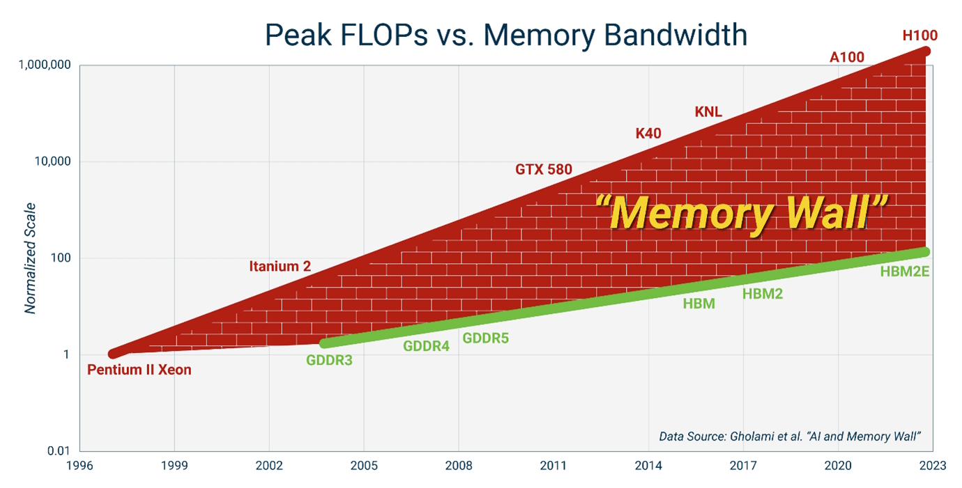
Before diving into how to predict memory access patterns, we need to understand why this problem is so critical. The answer lies in one of computer architecture’s most persistent challenges: the memory wall.
Modern processors can execute thousands of operations per cycle. But memory? Memory is slow. Accessing data from DRAM takes hundreds of cycles. If the processor has to wait for every memory access, it spends most of its time idle, waiting for data.
The solution has been a sophisticated memory hierarchy: small, fast caches close to the processor; larger, slower caches further away; eventually DRAM and storage. This hierarchy works beautifully when you can predict which data you’ll need next. Load it into cache before the processor asks for it, and the processor never has to wait. This is how architects fight the memory wall (Figure 1).
But how do you know what data to load?
Traditional Heuristics: Simple Patterns, Limited Reach
For decades, computer architects have used heuristic-based predictors. These are simple rules that capture common patterns:
Stride prefetchers detect when you’re accessing memory in regular patterns. If you access addresses 100, 104, 108, 112, the prefetcher notices the stride of 4 and starts loading 116, 120, 124 before you ask for them. This works beautifully for array traversals and simple loops, the bread and butter of traditional scientific computing.
Correlation prefetchers maintain a history of which addresses tend to follow which other addresses. If address A is often followed by address B, start loading B whenever you see A. This captures slightly more complex patterns than simple strides.
These heuristics work for regular, predictable access patterns. But modern workloads, especially AI workloads, are increasingly irregular. Sparse matrix operations, pointer-chasing through graph structures, hash table lookups, attention mechanisms in transformers. These patterns are much harder to capture with simple rules.
The fundamental limitation: Heuristics encode human intuition about common patterns. They work for patterns we’ve seen before and can articulate as simple rules. But what about patterns that are too complex for simple rules? What about workloads that don’t follow patterns we’ve seen before?
This is where machine learning becomes tempting. If we could learn memory access patterns rather than hand-coding heuristics, could we capture the complexity that traditional prefetchers miss?
The Promise and Challenge of Learning Memory Access Patterns
The paper “Learning Memory Access Patterns” (Hashemi et al., 2018) represents one of the most thorough attempts to apply deep learning to prefetching. It’s worth examining in detail because it reveals not just what machine learning can do for memory systems, but also the fundamental challenges that make this problem harder than it might seem.
The Core Idea: Memory Access as Sequence Prediction
The insight is elegant: treat memory access prediction as a sequence prediction problem. You have a history of addresses the program has accessed. Can you predict what addresses it will access next?
This maps naturally onto LSTM (Long Short-Term Memory) networks, which excel at sequence prediction. LSTMs have been remarkably successful at tasks like language modeling (predict the next word given previous words) and time series forecasting. The architecture seems like a perfect fit: feed in the sequence of past memory accesses, predict future accesses.
The paper proposes using LSTMs to replace traditional prefetchers entirely. Train the LSTM on memory access traces from real applications. Let it learn the patterns that humans would struggle to articulate as simple rules. Deploy it in hardware to predict which addresses to prefetch.
Why This Should Work
The case for learning seems obvious. Modern workloads have complex patterns: sparse matrices, graph traversals, pointer chasing through databases. These are too irregular for simple stride prefetchers. And ML has shown remarkable success with sequence prediction. Language models predict text with startling accuracy. Why not memory addresses?
Plus, workloads change over time. A learned prefetcher could adapt to new patterns that fixed heuristics miss. Retrain as applications evolve.
The intuition is powerful. But when you actually try to build this, you hit fundamental challenges that expose the limits of applying standard ML to systems problems.
Three Fundamental Challenges: Sparsity, Timing, and Heterogeneity
Try to build a learned prefetcher and you’ll hit three challenges that make memory prediction fundamentally different from other sequence prediction problems. These aren’t just engineering difficulties. They reveal why predictive reasoning in systems is harder than it looks.
Challenge 1: Sparsity (Learning from Signals Buried in Noise)
Here’s the first problem: only about 1% of memory addresses are accessed frequently enough to be worth predicting.
Think about what this means for learning. In language modeling, every word in your training data is potentially useful. Your vocabulary might be 50,000 words, and you’ll see most of them many times during training. The signal-to-noise ratio is high.
In memory access prediction, your “vocabulary” is the entire address space (potentially billions of addresses). But 99% of them are accessed so rarely that there’s nothing to learn. A few “hot” addresses dominate all the traffic. The rest is noise.
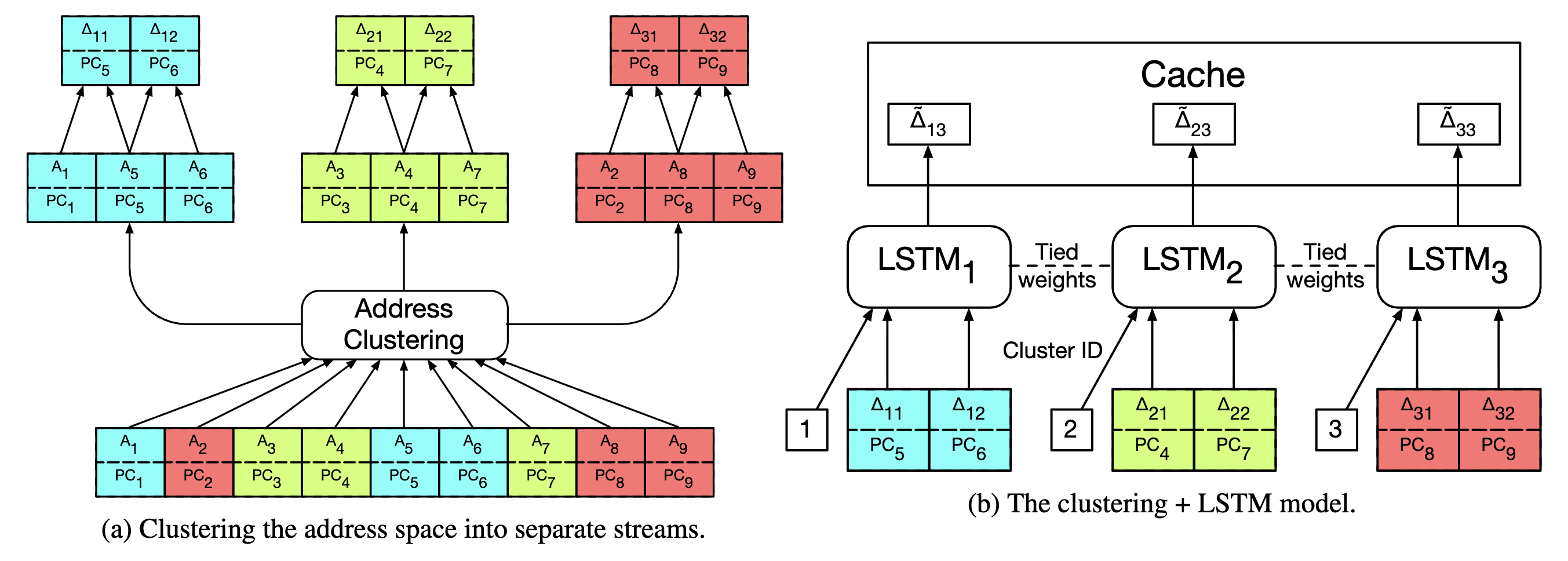
The Curse of Dimensionality in Address Spaces: When your vocabulary is the entire 64-bit address space (2^64 possible addresses), traditional one-hot encoding becomes impossible. You need 2^64 output neurons, which is absurd. The solution is typically to cluster addresses into regions or use hash-based representations. But this introduces its own problems: how do you cluster addresses when you don’t know which ones matter? The sparsity challenge appears at every level of the problem.
The paper uses delta encoding (predicting the difference between consecutive addresses rather than absolute addresses) to reduce the vocabulary. But even then, the sparsity remains. Most deltas occur rarely. A few dominate.
You’re trying to learn patterns from data where most of the data is uninformative. Standard ML assumes rich training signal. Here, signal is buried in noise.
The architecture must somehow focus on the small fraction of addresses that matter, ignore the vast majority that are noise, and do this dynamically as workloads change and different addresses become important.
Traditional ML metrics like accuracy become misleading. Predict “no prefetch” for everything and you’ll achieve 99% accuracy. Completely useless. The value comes from correctly predicting those rare, important accesses.
Challenge 2: Timing (When Prediction is as Important as What)
Here’s the second fundamental problem: prefetching is useless if your timing is wrong.
In most ML applications, timing doesn’t matter much. If your language model predicts the next word with a 100ms delay, that’s fine. If your image classifier takes 200ms instead of 100ms, you might not even notice.
Memory prefetching is different. The window for useful prediction is measured in nanoseconds to microseconds:
- Predict too early: Your prefetched data gets evicted from cache before the processor needs it. Wasted bandwidth, no benefit.
- Predict too late: The processor stalls waiting for data. Your prediction arrives after the processor already needed it.
- Predict just right: Data arrives in cache just before the processor needs it. This is the sweet spot.
Timeliness vs. Accuracy Trade-off: During our class discussion, students raised a crucial point: traditional prefetchers often optimize for coverage (what % of misses do you catch) and accuracy (what % of prefetches are used). But practitioners know that timeliness is equally critical. A prefetch that arrives one cycle too late is as useless as no prefetch at all. Yet most ML papers focus on what to predict, not when. The temporal dimension of prediction is systematically under-explored in the ML for systems literature.
Standard LSTM architecture has no notion of “when” to predict. It predicts the next item in the sequence, but doesn’t model timing. You could augment the model to predict both “what” and “when,” but that adds significant complexity.
The paper doesn’t fully solve this. The LSTM predicts what addresses will be accessed, but relies on heuristics to decide when to issue prefetches. This is a hybrid approach: learned model for “what,” heuristics for “when.”
Timing is a first-class constraint in systems. Most ML approaches treat it as secondary, just another input feature. But time is fundamental to whether your prediction has any value at all.
Challenge 3: Heterogeneity (One Model for Diverse Workloads)
The third challenge: different applications have completely different memory access patterns.
A matrix multiplication has regular, predictable strides. A graph traversal has irregular, pointer-chasing patterns. A hash table lookup has seemingly random access. A database workload mixes all of these and more.
If you train a model on one type of workload, will it generalize to others?
The paper evaluates across diverse benchmarks (SPEC CPU, graph workloads, etc.) and finds highly variable results. The LSTM works well on some workloads and poorly on others. There’s no single model that dominates across all application types.
You’re stuck choosing between bad options. Train specialized models per workload type? Now you need to classify workloads at runtime and switch models (complex and error-prone). Train one general model on diverse workloads? Mediocre performance everywhere. Use online learning to adapt dynamically? Training overhead during execution.
None of these is clearly superior. Each involves trade-offs that depend on your deployment constraints.
Here’s the deeper issue: heterogeneity is fundamental to systems. Unlike image classification (where all inputs are images) or language modeling (where all inputs are text), systems workloads are inherently diverse. A prefetcher can’t assume its workload will look like its training data.
Learned Index Structures: When Patterns Are Stable
While prefetching wrestles with sparsity and timing, there’s another area where machine learning has shown more clear-cut success: learned index structures.
The paper “The Case for Learned Index Structures” (Kraska et al., 2018) made a provocative claim: you can replace traditional data structures like B-trees, hash tables, and Bloom filters with learned models. When data has patterns, ML can exploit those patterns more efficiently than generic data structures designed to work for any data distribution.
The Core Insight: Data Structures as Models
Traditional data structures make no assumptions about your data. A B-tree works whether your data is uniformly distributed, skewed, sorted, or random. O(log n) lookup time regardless of data distribution.
But this generality has a cost. If your data has structure (timestamps that increase monotonically, user IDs that cluster by region), a B-tree doesn’t exploit that structure. It treats your data as if it could be arbitrary.
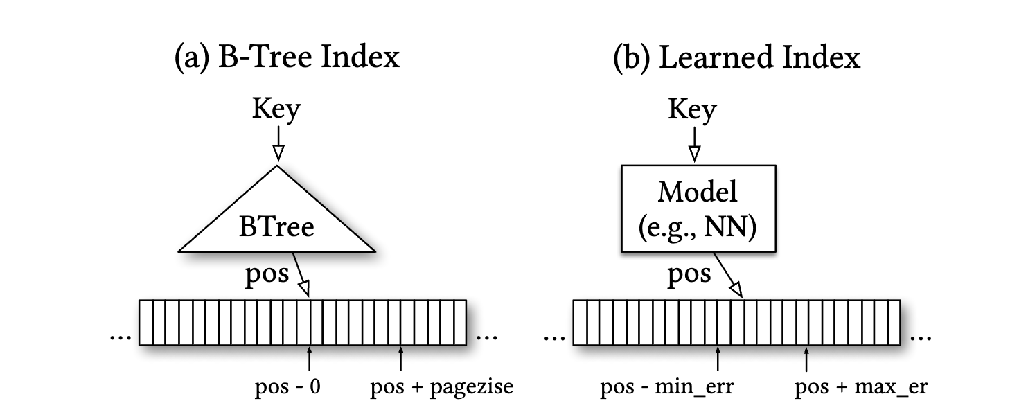
Here’s the insight: an index is really just a model of your data distribution. Given a key, where is it located? That’s a prediction problem. For a sorted array of n elements, it’s learning the cumulative distribution function (CDF): what fraction of keys are less than this key?
If you can learn the CDF, you can predict where a key is located. Then you only need a small correction (binary search over a small range) to find the exact position.
For example, if you’re indexing 1 billion user records by timestamp spanning January 1 to December 31, a learned model could predict: “timestamp for March 15 is approximately at position 250 million” (roughly 1/4 through the year). Then you do a local search within a small range around position 250 million.
This can be much faster than traversing a B-tree, especially when your learned model is simple and exploits data distribution structure as shown in Figure 3.
Why Google Cared About This
Before diving into results, consider why Google invested in this research. At Google’s scale, even small improvements compound dramatically. When you’re serving billions of queries per day across systems like BigTable, Spanner, and search infrastructure, a 2-3x speedup translates to massive cost savings in compute and power. More importantly, a 10-100x reduction in memory footprint means you can fit indices that previously required hundreds of servers onto dozens, directly impacting datacenter costs.
Many of Google’s core workloads fit the learned index sweet spot: read-heavy with stable data distributions. Search indices don’t change drastically hour-to-hour. Ad targeting data has clear patterns (users from certain regions, certain age groups, certain interests). These workloads are exactly where you can train once and serve billions of queries, amortizing the training cost over massive inference volume.
The paper came from Google researchers (Kraska worked closely with Jeff Dean’s team) precisely because they had both the motivation (scale) and the right workloads (stable patterns, read-heavy) to make learned indexes worthwhile.Jeff Dean is one of Google’s most influential engineers, leading Google AI and co-designing foundational systems like MapReduce, BigTable, Spanner, and TensorFlow. He’s also known for “Latency Numbers Every Programmer Should Know”, a list that makes explicit the performance costs we discussed (DRAM access: 100ns, SSD read: 150μs). His team’s investment in learned index structures reflects a broader vision: using ML not just for applications, but to optimize the infrastructure itself. When Dean’s group explores an idea, it’s usually because they’ve identified a real pain point at Google’s scale that could save millions in operational costs. This wasn’t academic curiosity. It was solving a real infrastructure cost problem.
When This Works: The Power of Patterns
The results are striking. For datasets with strong patterns (sorted data, clear correlations), learned indexes can be 2-3x faster than B-trees for lookups, 10-100x smaller in memory footprint, and more cache-efficient.
Real-world data often has patterns. Timestamps are ordered. User IDs correlate with geographic regions. Product IDs cluster by category. These patterns are exploitable.
Learned indexes can also combine multiple features. Traditional indexes work on a single key. A learned index could use multiple correlated attributes: “Users from California tend to have IDs in this range and registration dates around this time.” The model learns joint distributions.
The Limitation: When Patterns Change
But there’s a fundamental limitation: what happens when your data changes?
A B-tree handles insertions and deletions dynamically. Add a new key, and the tree structure updates. The data structure maintains its guarantees regardless of how data evolves.
A learned index faces the retraining problem. Your model learned the CDF of your current data. Add new data, and the CDF changes. Now your predictions are wrong. You need to retrain.
For workloads where data is largely static (read-heavy databases, data warehouses, log archives), this isn’t a problem. Train once, serve forever. The learned index dominates.
For workloads where data changes frequently (write-heavy databases, real-time systems), retraining overhead becomes significant. You could periodically retrain (accumulate changes, retrain offline, deploy new model, but predictions go stale). Or use online learning (update continuously, but that adds overhead to every write). Or build hybrid structures (learned models for stable data, traditional structures for recent changes, the approach ALEX explores).
Here’s the core tension: ML excels at exploiting patterns in static data. But systems are dynamic. Data changes. Workloads evolve. How do you maintain learned models in the face of continuous change?
The Tacit Knowledge: Predictive Reasoning Under Uncertainty
Both prefetching and learned indexes expose a common challenge. Think about it: when you’re designing a memory system, there’s no way to fully characterize all the workloads that will run on it. You don’t know what applications people will write. When deploying a learned index, you don’t know exactly how your data distribution will evolve. You’re making bets about future behavior with incomplete information.
This is predictive reasoning: designing systems that work well across scenarios you haven’t fully observed, making informed judgments about which patterns are worth optimizing for and which risks are worth taking.
This is tacit knowledge because it’s not in the papers. The papers tell you how LSTM prefetchers work or how learned indexes achieve speedups on benchmarks. But they don’t tell you when to use learned prefetching versus traditional heuristics. How to know if your workload has patterns worth learning. What balance between specialization and generality. When retraining overhead is worth the benefit. How to design for workloads you haven’t seen yet.
Experienced architects develop intuition about these questions through building many systems. They’ve seen which patterns are common across workloads. They understand when prediction overhead pays off. They know how to design systems that degrade gracefully when predictions fail.
How This Differs from Co-Design Reasoning
Last week, we examined co-design reasoning: optimizing interdependent constraints simultaneously. Everything depends on everything else.
Predictive reasoning is different. It’s not about interdependence. It’s about incomplete information.
In co-design, if you had perfect information about the workload, hardware, and constraints, you could compute the optimal solution (though it might be computationally expensive). The challenge is circular dependencies.
In prediction, even with complete information about past workloads, you don’t know future workloads. Even with perfect models of current data distributions, you don’t know how distributions will change. The challenge is irreducible uncertainty.
This requires different strategies. Design for robustness over optimality (work reasonably well across diverse scenarios rather than optimally for one). Build adaptation mechanisms that adjust to changing patterns rather than assuming static environments. Have fallback strategies for when predictions fail. Understand the cost of being wrong and design accordingly.
These aren’t skills you learn from reading papers. They’re developed through experience: seeing which predictions hold up in production and which don’t, understanding how workloads evolve, learning when adaptation overhead pays off.
Industry Perspective: What Actually Works in Production
 Milad Hashemi is a Research Scientist at Google working on the ML, Systems, and Cloud AI team. As lead author of the “Learning Memory Access Patterns” paper we discussed, he brings first-hand experience with both the promise and practical challenges of applying ML to low-level systems. His work bridges the gap between academic research and production deployment, understanding both what works in papers and what survives contact with real-world constraints.
Our guest speaker this week, Milad Hashemi, provided crucial context about what happens when learned memory systems meet production reality. The gap between research results and deployed systems reveals much about where predictive reasoning remains fundamentally hard.
The Retraining Bottleneck
One of the first questions from class addressed the elephant in the room: “If I need to retrain my model every time I add new data, doesn’t that kill the benefits?”
Milad’s response was candid: this is exactly why learned index structures haven’t seen widespread production adoption despite impressive benchmark results. The retraining problem is more severe than papers often acknowledge.
In research settings, you train once on a fixed dataset and measure performance. In production, data evolves continuously. New users sign up. Products get added to catalogs. Log entries accumulate. The data distribution shifts.
For learned indexes, this means your CDF model becomes stale. Predictions drift. Performance degrades. You need to retrain. But retraining has costs: computational overhead (training neural networks isn’t free at scale), service disruption (take the index offline or serve stale predictions?), and coordination complexity (coordinate model updates across many nodes in distributed systems).
The result? Production systems often stick with traditional data structures that handle updates dynamically, even if they’re slower in the steady state. Predictability and consistency often trump raw performance in production.
A key aspect of predictive reasoning: it’s not just about making accurate predictions. It’s about making predictions that remain accurate as the world changes, with update mechanisms that don’t disrupt service.
When Learned Systems Win: The Static Data Niche
But Milad also highlighted where learned approaches genuinely shine: read-heavy workloads over largely static data.
Data warehouses with append-only logs analyzed for insights (data distribution changes slowly). CDNs and caches where content popularity follows power-law distributions that stay relatively stable. ML serving where model weights don’t change during inference and access patterns are consistent.
In these domains, you can amortize training costs over millions or billions of queries. The patterns are stable enough that models stay accurate. The workloads are homogeneous enough that a single model works well.
Several large-scale systems at Google have adopted learned approaches for these specific niches. The key is choosing workloads where the assumptions (static data, homogeneous patterns, read-heavy) actually hold.
Experienced practitioners know how to recognize these niches. They understand which workload characteristics make learning worthwhile versus where traditional approaches are safer. This pattern recognition comes from seeing many systems in production.
The Heterogeneity Problem in Practice
Class discussion also surfaced a critical observation from the transcripts: “Different parts of your application might need completely different prefetching strategies.”
In a modern server handling web requests, you might simultaneously be serving cached static content (predictable access patterns), processing database queries (irregular pointer chasing), running ML inference (regular tensor operations), and handling authentication (hash table lookups). Each has different memory characteristics. A single learned prefetcher struggles with this diversity.
The practical solution is often hybrid approaches: use traditional heuristics as the base, add learned components for specific patterns you identify. This requires infrastructure to classify workload phases at runtime, switch between prediction strategies, and fall back gracefully when learned models fail.
Building this infrastructure is engineering-heavy work that research papers rarely discuss. But it’s where much of the real complexity lives in production systems.
The Generative AI Question: Can Modern LLMs Help?
During class, students raised a provocative question: “We’re talking about LSTMs from 2018. Could modern generative AI (transformers, LLMs) do better at prefetching?”
This question is sharper than it might initially seem. It forces us to think carefully about what generative models actually offer and whether those capabilities address the fundamental challenges we’ve identified.
What Transformers Might Offer
There are genuine reasons to be intrigued. Transformers handle long sequences better. LSTMs struggle beyond a few hundred elements, while transformers with attention can model dependencies across much longer contexts. They’re more parallelizable, which could reduce prediction latency. Pre-trained models might transfer better across workloads, learning general patterns about memory access the way LLMs learned general patterns about language. And GPT-style models work across diverse text domains without retraining. Maybe they could similarly handle diverse memory access patterns.
These are legitimate possibilities. But we need to confront the fundamental barriers:
The Fundamental Barriers
The timing problem doesn’t go away. Transformers are slower than LSTMs for inference, not faster. A prefetcher needs to make predictions in nanoseconds. Even a tiny transformer takes orders of magnitude longer. Unless you’re doing batch prediction (which breaks the online nature of prefetching), the latency is prohibitive.
As noted during discussion: “Generative AI might slow down the system despite its benefits.” For prefetching, latency is not negotiable. You can’t prefetch 1000 cycles late because your model is still computing attention weights.
The sparsity challenge remains. Transformers are data-hungry. They typically need millions of training examples. Memory access traces are sparse by nature (99% noise, 1% signal). Standard transformer training assumes dense, meaningful data. The architectural mismatch persists.
The semantics gap is crucial. One student observation from the transcript was particularly insightful: “The importance of semantics in data for effective prefetching.” Memory addresses are just numbers. They don’t have the rich semantic structure that language has. In language, “king” and “queen” have semantic relationships that embeddings can capture. Memory addresses? Much less so.
LLMs succeed partly because language has rich compositional semantics. Memory addresses are largely arbitrary. Address 0x7ff3a840 has no semantic relationship to 0x7ff3a844 unless you understand the program’s data structures. And that understanding isn’t in the addresses themselves.
A More Promising Direction: Software-Coupled Prediction
However, one direction from the discussion seems genuinely promising: “Coupling prefetching with software attributes, the actual algorithm or code executing.”
Instead of predicting from raw memory addresses, what if you incorporated:
- Code context: What function is executing? What loop are we in?
- Algorithm semantics: Is this a matrix multiplication? Graph traversal? Hash lookup?
- Type information: What data structures are being accessed?
- Program phase: Are we in initialization? Steady state computation? Cleanup?
This is actually closer to what compilers and profilers do. They have semantic understanding of the program, not just observed memory traces.
This is where LLMs might genuinely help. Recent work on “Performance Prediction for Large Systems via Text-to-Text Regression” shows that encoder-decoder models can predict system performance from configuration files and system logs, exactly the kind of rich semantic context that raw memory traces lack. For Google’s Borg cluster scheduler, a 60M parameter model achieves near-perfect 0.99 rank correlation in predicting resource efficiency. The key insight as shown in Figure 4: treat system prediction as a text understanding problem rather than pure numerical regression.
Not by replacing hardware prefetchers, but by understanding code and suggesting where software prefetch hints should be inserted. The LLM operates at compile time or development time, with access to full program context, no timing constraints, and rich semantic information.

This is less sexy than “LLMs do prefetching” but potentially more practical: LLMs augment human understanding of memory behavior, helping developers optimize memory access patterns at the software level.
What This Means for AI Agents
Throughout this exploration of memory systems, we’ve encountered predictive reasoning challenges that expose fundamental limitations in current AI approaches to systems design.
What would AI agents need to master predictive reasoning? Let’s synthesize:
Challenge 1: Learning from Sparse Signals
Current ML assumes abundant data where most examples are informative. Memory systems have the opposite: 99% noise, 1% critical signal.
What agents need: The ability to identify and focus on rare but important events, ignoring the vast majority of data that’s uninformative. This isn’t just about class imbalance (which ML has tools for). It’s about fundamental sparsity where the “vocabulary” is enormous but only a tiny fraction matters.
Current gap: Standard architectures (transformers, LSTMs) are designed for relatively dense feature spaces. Adapting them to extreme sparsity remains an open challenge.
Challenge 2: Temporal Reasoning as First-Class
Timing isn’t just another feature you can feed into a model. It’s a fundamental constraint that determines whether predictions are useful at all.
What agents need: Integrated reasoning about “what” to predict and “when” predictions matter. Not just sequence modeling, but causal timing models that understand latency constraints and temporal windows of opportunity.
Current gap: Most ML treats time as just another input dimension. Systems need time as a first-class constraint that shapes the entire prediction task.
Challenge 3: Heterogeneity and Transfer
A single agent must handle workloads ranging from regular matrix operations to irregular graph traversals, without knowing in advance which pattern it will encounter.
What agents need: Meta-learning that can identify which patterns are present in a workload and adapt prediction strategies accordingly. Not just multi-task learning, but online recognition of workload characteristics.
Current gap: Current approaches either specialize (train per workload) or generalize poorly (one model, mediocre everywhere). Effective online adaptation remains elusive.
Challenge 4: Dynamic World Modeling
Systems aren’t static. Data distributions change. Workloads evolve. Access patterns shift.
What agents need: Mechanisms for updating predictions as the world changes, with minimal overhead and without service disruption. Detecting when distributions have shifted enough to warrant retraining. Incremental learning that updates models efficiently. Graceful degradation when predictions become stale.
Current gap: Most ML assumes train-once-serve-forever or expensive periodic retraining. Efficient online adaptation for low-level systems remains challenging.
Challenge 5: Risk-Aware Decision Making
Being wrong has immediate costs (cache pollution, wasted bandwidth, processor stalls). Not all prediction errors are equal.
What agents need: Understanding of cost functions where false positives and false negatives have very different costs, and where the cost structure depends on system state (cache occupancy, bandwidth utilization, processor workload).
Current gap: Standard ML loss functions don’t capture the system-level costs of different types of errors. Incorporating these into learning is non-trivial.
The Broader Pattern: Predictive Reasoning Across Systems
Predictive reasoning under uncertainty isn’t unique to memory systems. It appears throughout computer systems design.
Network traffic prediction demands forecasting bandwidth needs and congestion patterns for routing algorithms, but you’re designing for traffic you haven’t seen, with tight timing constraints. Power management requires predicting future CPU utilization to decide whether to sleep cores (wrong predictions waste power or hurt performance). Cloud resource allocation needs predicting VM resource needs for optimal placement, but workloads are heterogeneous and patterns change. Storage caching faces similar challenges to memory prefetching, just at different timescales.
The pattern repeats: sparse signals, heterogeneous workloads, timing constraints, dynamic environments. Architects must design systems for patterns they can’t fully characterize.
What separates experienced architects from novices? Recognizing when patterns are stable enough to learn versus when simple heuristics are more robust. Knowing how to design systems that degrade gracefully when predictions fail. Understanding which workload characteristics generalize across applications.
Looking Forward: Week 10 and Beyond
We’ve now explored two types of tacit architectural knowledge:
Week 8: Co-design reasoning (handling circular dependencies where everything depends on everything else).
Week 9: Predictive reasoning (designing for patterns you can’t fully observe or characterize).
Next week: adaptive reasoning. LLM serving systems must dynamically schedule requests, manage memory, and balance throughput versus latency, all while conditions continuously change. You can’t just predict. You must continuously adapt.
This builds directly on this week’s themes. The same memory management challenges we discussed (KV-cache, attention patterns) appear in LLM systems. But now we add real-time decision making under load.
Each week reveals another facet of what “architectural thinking” means. These are the skills that experienced architects have developed through years of building systems. They’re also the skills that AI agents must somehow develop to become true co-designers.
The question isn’t whether AI will replace human architects. It’s whether we can help AI agents develop these different types of reasoning, each with its own challenges and characteristics. And whether human-AI collaboration can combine the strengths of both: AI’s systematic exploration with human judgment and intuition.
Questions for Reflection
For researchers: How do we build ML systems that learn from sparse signals with timing constraints? Can we develop architectures specifically designed for system prediction tasks rather than adapting NLP/vision models?
For practitioners: When should you invest in learned approaches versus traditional heuristics for memory systems? How do you evaluate whether your workload has patterns worth learning?
For educators: How do we teach predictive reasoning under uncertainty? What abstractions help students develop intuition about when patterns are stable enough to exploit?
For the field: What other domains in computer systems require this type of predictive reasoning? How do we build benchmarks and evaluation methodology that capture the real-world challenges (sparsity, timing, heterogeneity) that make prediction hard?
The deeper question: Can AI agents learn to recognize which patterns are worth predicting, or will this always require human judgment? When a learned prefetcher outperforms heuristics on benchmarks but fails in production, how do we help agents understand why?
For detailed readings, slides, and materials for this week, see Week 9 in the course schedule.