Week 8: Can AI Master Co-Design Reasoning? When Everything Depends on Everything
Last week, we confronted an important challenge: architectural knowledge is tacit. It exists in the minds of experienced computer architects, accumulated through decades of building systems. We saw how this creates an epistemological problem for AI agents trying to become co-designers.
But what exactly IS this tacit knowledge? When we say architectural expertise is “tacit,” what specifically are we talking about?
The answer isn’t simple. Tacit knowledge isn’t a single thing. It’s a collection of different types of reasoning that architects have developed through experience. In this series, we examine these different types one by one, using concrete problems to make each type visible and understandable.
Today, we examine the first type: co-design reasoning. This is the ability to reason about interdependent constraints simultaneously. You cannot optimize one aspect without considering how it affects everything else.
Why does this matter for AI agents? Because most real-world design problems involve interdependent choices. From designing distributed systems to optimizing compilers to architecting chips, you can’t decompose the problem into independent subproblems. Current AI approaches struggle with this. They excel at pattern matching within fixed problem structures but falter when the problem structure itself is part of what needs to be designed.
We’ll use the mapping problem as our window into this type of reasoning, exploring what makes it challenging and what fundamental capabilities AI agents would need to master it.
What Is Mapping?
Mapping is the decision of how computation gets executed on hardware.For a thorough technical treatment of AI hardware mapping fundamentals, including computation placement, memory allocation, and combinatorial complexity, see the Hardware Mapping Fundamentals for Neural Networks chapter in the Machine Learning Systems textbook. It’s the bridge between what you want to compute (the algorithm) and how the hardware actually performs that computation.
Consider a simple example: multiplying two matrices. The mathematical operation is well defined. But when you implement it on an accelerator, you face hundreds of concrete decisions:
- Should you process the matrices row by row or column by column?
- How do you break the large matrices into smaller chunks that fit in fast memory?
- Which data should you keep in cache versus reload from slow memory?
- In what order should you perform the operations?
- How do you distribute the work across multiple compute units?
Each of these decisions is a mapping choice. The same matrix multiplication, on the same hardware, can have billions of different mappings. Most perform poorly. A few achieve near optimal efficiency.
This matters because modern AI accelerators are incredibly fast at computation but relatively slow at moving data. The mapping determines how much data movement you need. Get it wrong, and your expensive hardware sits idle, waiting for data. Get it right, and you achieve orders of magnitude better performance.
We’ll make this concrete shortly with a detailed example. But first, why is mapping particularly interesting for studying co-design reasoning?
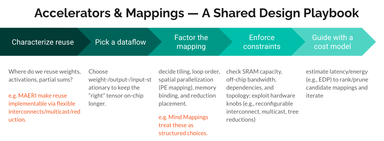
As a useful mental model, see Figure 1, which frames mapping within a broader systems optimization playbook—sitting between workload characteristics and hardware execution.
Why Mapping? The Architecture Design Challenge
Why did we choose mapping as the problem to illustrate co-design reasoning? Because when AI agents design architectures, they must reason about mapping simultaneously.
The stakes are high. Remember Week 5’s discussion of GPU performance engineering: getting peak performance from hardware requires understanding how your computation maps onto the architecture. The difference between a naive mapping and an optimized one can be 10-100x in performance. At scale, this difference translates to millions of dollars in infrastructure costs and determines what applications are even feasible to run. Mapping isn’t just an academic exercise. It’s the difference between a successful product and an unusable one.
Consider typical software optimization scenarios (this was Phase 1):
- CPU optimization: Software changes, hardware is fixed
- GPU kernels: Write code to match fixed hardware
- Distributed systems: Map workloads to existing infrastructure
In each case, one side is fixed. You’re optimizing within constraints.
Architecture design is fundamentally different. When you’re designing a new accelerator, you’re not just finding the best mapping for fixed hardware. You’re deciding what hardware to build in the first place. And you can’t make that decision without understanding how workloads will map onto it.
This creates a co-design challenge:
- The hardware architecture (memory hierarchy, interconnects, compute units)
- The mapping strategies (how computations map onto that architecture)
- The workload characteristics (what algorithms need to run efficiently)
You cannot design the architecture without understanding the mapping. A 256KB cache looks great until you realize your target workloads need 512KB for efficient tiling. You cannot optimize the mapping without knowing the architecture. Those 32×32 tiles are perfect for one memory hierarchy but terrible for another.
What makes mapping particularly interesting is that even with fixed hardware and software, the mapping space itself is vast (billions of configurations). When the hardware itself is ALSO a design variable, the interdependencies multiply. An AI agent designing architectures must reason about: “If I make the cache this size, what mappings become possible? If I optimize for these mappings, what does that imply about the hardware I should build?”
This triple malleability creates interdependencies that are fundamentally different from traditional optimization problems. We now examine these interdependencies through a concrete example.
Making Mapping Concrete: The Tiling Problem
Modern AI accelerators have tensor cores capable of performing thousands of operations per cycle. But these tensor cores spend most of their time idle, waiting for data. The “memory wall”The Memory Wall: Sally McKee’s seminal 1995 paper “Hitting the Memory Wall: Implications of the Obvious” quantified how processor speeds doubled every 18 months while DRAM access times improved only 7% annually, creating a fundamental performance gap. McKee, a pioneering computer architect who passed away in 2024, spent her career advancing memory system design. Thirty years later, this bottleneck has only intensified: computation is cheap, but data movement is expensive. means the problem isn’t compute capacity. It’s moving data from memory to the compute units fast enough to keep them fed.
To understand what mapping actually entails, we examine matrix multiplication as our concrete example. Matrix operations form the backbone of most deep learning computations.
The central challenge is tiling (or blocking): breaking large matrices into smaller submatrices that fit in faster memory levels. Think of it like handling a giant jigsaw puzzle by working on smaller sections at a time. Different tiling strategies lead to different memory access patterns and dramatically different performance.
Suppose you have:
- A simple matrix multiplication:
C = A × B - An accelerator with tensor cores that operate on small tiles (say, 16×16 matrices)
- A memory hierarchy: small fast cache, large slow DRAM
The mapping question: How do you tile your large matrices to efficiently use your tensor cores?
This requires making four interrelated decisions:
First Decision: Which Loops to Tile?
Matrix multiplication has three nested loops (over rows of A, columns of B, and the shared dimension). You could tile any combination of them. Each choice creates different memory access patterns.
Consider the basic loop structure:
# Naive matrix multiplication: C = A × B
for i in range(M):     # rows of A
    for j in range(N):    # columns of B
        for k in range(K):  # shared dimension
            C[i,j] += A[i,k] * B[k,j]
Now you want to tile this for your 16×16 tensor cores. Which loops do you tile? Here’s one choice:
# Tiled version: process 16×16 blocks
for i_tile in range(0, M, 16):
    for j_tile in range(0, N, 16):
        for k_tile in range(0, K, 16):
            # Process 16×16×16 tile
            for i in range(i_tile, i_tile+16):
                for j in range(j_tile, j_tile+16):
                    for k in range(k_tile, k_tile+16):
                        C[i,j] += A[i,k] * B[k,j]
But you could tile in different ways (tile only i and j, different tile sizes, different loop orders). Each creates different memory access patterns.
Second Decision: What Tile Sizes?
Suppose you choose to tile all three dimensions. What size tiles? The space is enormous. For a 1024×1024 matrix multiplication with tensor cores operating on 16×16 tiles, you have billions of possible tiling configurations.
This depends on:
- Your tensor core size (hardware constraint): 16×16 means tiles should be multiples of 16
- Your cache size (hardware constraint): A 256KB L1 cache can hold roughly 32K float32 values
- Your memory bandwidth (hardware constraint): Can you feed data fast enough to saturate compute?
- The size of your input matrices (workload constraint): Different matrices have different optimal tile sizes
Third Decision: Which Data in Which Memory?
You have multiple levels of memory hierarchy (registers, L1 cache, L2 cache, DRAM). Which tiles of A, B, and C belong in which level?
This depends on:
- How often each tile is reused
- How big each tile is
- What your memory capacities are
- What your dataflow pattern is
Fourth Decision: What Dataflow Pattern?
Dataflow patterns describe which data stays put (stationary) and which data moves through the accelerator. Output stationary keeps partial results (outputs) in place while streaming inputs (good when outputs are reused many times). Weight stationary keeps model parameters (weights) in place while streaming activations (good when the same weights are applied to many inputs). Input stationary keeps input activations in place (useful for certain convolution patterns). The choice fundamentally affects memory traffic, energy, and achievable performance. For a comprehensive treatment of data movement patterns and dataflow optimization strategies, see the Machine Learning Systems textbook.
Do you:
- Stream rows of A and columns of B past stationary tiles of C? (output stationary)
- Stream tiles of C past stationary tiles of A and B? (weight stationary)
- Some hybrid approach?
This depends on:
- Your memory bandwidth
- Your compute pattern
- Which data has the most reuse
- What your hardware interconnect looks like
The crucial insight: Each of these decisions depends on the others.
The Circular Dependency
What does this mean for AI agents? Traditional machine learning assumes you can decompose problems into independent subproblems or optimize sequentially. Train a model to choose tile sizes. Train another to select dataflow. Combine the outputs. But mapping doesn’t work this way.
The optimal choice for any single decision depends on what you choose for all the others. You cannot train separate models and combine their outputs. You cannot fix one variable and optimize the rest. The circular dependencies force agents to reason about the entire problem simultaneously.
This is Challenge 1: reasoning about circular dependencies. Problems where you cannot decompose into independent subproblems.
Most machine learning frameworks assume you can define a clear objective function and search for solutions that maximize it. But here, evaluation itself is circular. You can’t judge whether a solution is “good” without simultaneously considering hardware design, software structure, and mapping choices. The evaluation function depends on design decisions you haven’t made yet.
Let’s trace through these circular dependencies in concrete terms:
Can’t choose tile sizes without knowing memory hierarchy: If you have 256KB L1 cache, should you use 32×32 tiles (storing 3×1024 values) or 64×64 tiles (storing 3×4096 values)? The answer depends on how many tiles you need active simultaneously. But that depends on your dataflow pattern.
Can’t design memory hierarchy without knowing access patterns: How much cache do you need? If your dataflow reuses output tiles extensively, you need larger cache. If it streams everything, cache size matters less. But which dataflow should you assume? That depends on your memory bandwidth constraints.
Can’t determine access patterns without knowing dataflow: Output stationary keeps C tiles in cache, reading each A and B element once (high reuse of outputs). Weight stationary keeps A or B in cache, streaming C tiles (high reuse of weights). These have 10-100x different memory traffic patterns. But which should you choose? That depends on whether you’re memory-bound or compute-bound.
Can’t choose dataflow without knowing memory bandwidth: If your memory bandwidth is 900 GB/s but your compute can consume 19.5 TFLOPS (like an NVIDIA V100), you’re severely memory-bound. This demands output-stationary dataflow to maximize reuse. But that constrains your tile sizes to fit output tiles in cache.
Can’t predict memory bandwidth utilization without knowing tile sizes: Larger tiles mean fewer memory transactions but risk cache thrashing. Smaller tiles mean more overhead but better locality. The optimal balance depends on your memory hierarchy design.
Can’t choose tile sizes without knowing memory hierarchy…
We’re back where we started. This is a circular dependency. Every decision constrains and is constrained by every other decision.
Hierarchy] B --> C[Access
Patterns] C --> D[Dataflow] D --> E[Bandwidth] E --> A style A fill:#2563eb,color:#fff style B fill:#dc2626,color:#fff style C fill:#9333ea,color:#fff style D fill:#16a34a,color:#fff style E fill:#ea580c,color:#fff
This is what makes co-design reasoning fundamentally different from the optimization we did in Phase 1. In Phase 1, we had clear constraints we could optimize within. Here, the constraints themselves are interdependent design choices that must be reasoned about simultaneously.
This is tacit knowledge. Remember Week 7’s central question: how do AI agents learn what was never written down? Here’s a concrete example. An experienced architect might look at a workload and immediately say: “Use output-stationary dataflow with 32×32 tiles.”
The knowledge isn’t categorical rules like “32×32 tiles are good.” It’s relational understanding. How do tile sizes interact with cache capacity under specific bandwidth constraints? How do dataflow choices affect memory traffic by 10-100x? Why do certain patterns work for certain workload characteristics? This knowledge spans hardware (cache hierarchy), software (loop structure), and physics (memory latency). It’s developed through building many systems and seeing what works.
You can’t easily codify it as rules or learn it by showing examples, because the “best” solution is deeply context-dependent. This is Challenge 2: context-dependent knowledge transfer. Understanding not just “what works” but “when and why it works.”
Supervised learning can’t just memorize solutions. Reinforcement learning can’t randomly explore 10^15 configurations. This is Challenge 3: sample efficiency under massive search spaces. The circular structure means you need new approaches.
Two Approaches to Co-Design Reasoning
How do we help AI agents develop this type of reasoning? We examine two papers that illustrate fundamentally different approaches to the mapping problem. These aren’t comprehensive solutions. They’re examples chosen to reveal what co-design reasoning requires and expose gaps in current capabilities. One takes an analytical approach, encoding relationships explicitly. The other learns from experience. Both show different aspects of what AI agents would need to master.
DOSA: Encoding Relationships as Differentiable Models
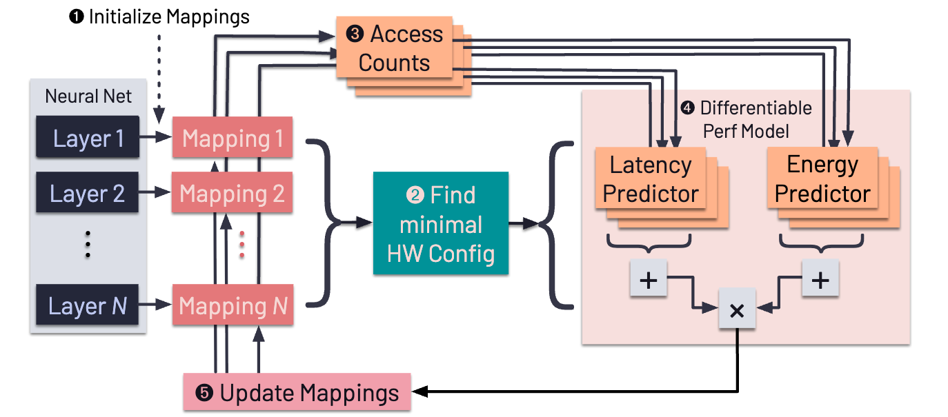
DOSA (Differentiable Model-Based One-Loop Search for DNN Accelerators) takes an analytical approach: encode the relationships between hardware and mapping as differentiable mathematical equations. Figure 2 illustrates the DOSA architecture and its joint exploration of hardware and mapping spaces via a differentiable performance model.
The core insight: if you can model how changing hardware parameters affects mapping quality, and how changing mapping affects hardware utilization, you can use gradient descent to explore the coupled space.
DOSA builds on TimeLoopTimeLoop is an infrastructure for evaluating and exploring the architecture design space of deep neural network accelerators. Developed at NVIDIA and MIT, it models the data movement and compute patterns of DNN workloads mapped onto hardware architectures, predicting energy consumption and performance. TimeLoop has become a standard tool in academic and industrial accelerator research, encoding decades of knowledge about how to model accelerator behavior accurately., an analytical performance model that predicts latency and energy for DNN accelerators. TimeLoop encodes years of expert understanding about how accelerators work: memory access costs, compute throughput, interconnect constraints.
What DOSA reveals about what AI agents need:
First, agents must understand RELATIONSHIPS between choices, not just evaluate individual choices. When you change tile size, it affects memory pressure, which affects bandwidth utilization, which affects compute occupancy. DOSA encodes these relationships explicitly as mathematical equations. An agent working from scratch would need to discover or learn these relationships.
Second, when you CAN model the interdependencies, you can exploit structure. Gradient descent works because the relationships are smooth enough that local improvements lead toward global improvements. This is exploiting the structure of the problem.
Third, sample efficiency matters. DOSA achieves 0.1% error compared to detailed simulation, but with orders of magnitude fewer evaluations than black-box search methods like Bayesian optimization. Consider the scale: the design space for a realistic accelerator has on the order of 10^15 possible configurations. Even evaluating one million designs samples only 10^-9 of the space. When you can’t afford to try millions of design points, encoding domain knowledge becomes essential.
The limitation: This requires being able to model the relationships analytically. TimeLoop represents decades of collective architectural knowledge, hand-crafted by experts. Building such models is expensive and requires deep domain expertise.
AutoTVM: Learning from Experience
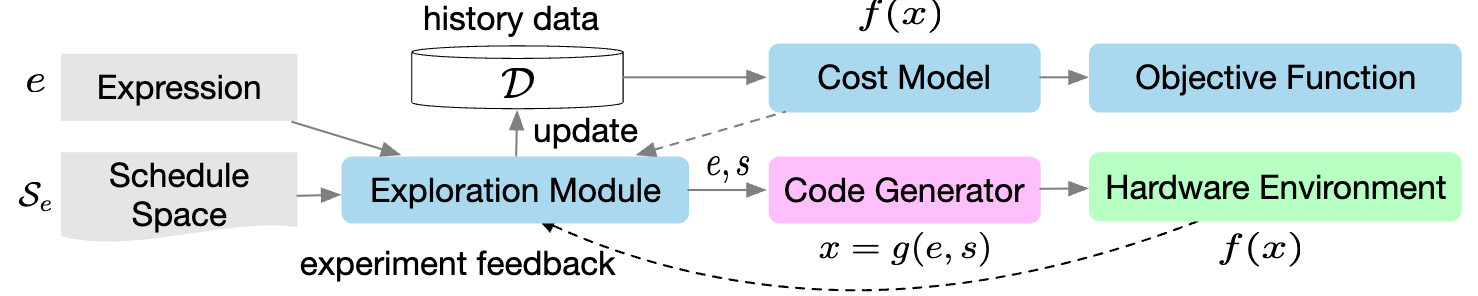
AutoTVM (Learning to Optimize Tensor Programs), part of Apache TVM, takes a learning approach: explore many mappings, learn patterns about what works, and generalize to new workloads. Figure 3 shows how AutoTVM explores program variants guided by a statistical cost model.
The core insight: even though we can’t analytically model all the relationships, we can learn from experience what types of mappings work well for what types of workloads.
AutoTVM generates a space of possible mappings (through templates that structure the search space), tries many of them, builds a performance predictor, and uses that predictor to guide further search.
What AutoTVM reveals about what AI agents need:
First, agents need pattern recognition capabilities. Instead of reasoning from first principles about every mapping, an agent should recognize “this workload is similar to ones I’ve seen before, and this TYPE of mapping worked well there.” This is where machine learning excels.
Second, transfer learning is crucial. Knowledge learned from optimizing one workload helps with similar workloads. Co-design reasoning isn’t just about memorizing “this specific mapping works.” It’s about abstraction: “mappings with these characteristics work for workloads with these properties.”
Third, you need structure even when learning. AutoTVM doesn’t search the raw space of all possible code transformations. It uses templates that encode reasonable search spaces. Even learning-based approaches need some domain structure.
The limitation: This requires many samples to learn from. While more sample-efficient than random search, it still needs substantial exploration. And the learned knowledge doesn’t necessarily transfer across very different architectures.
The Synthesis
DOSA and AutoTVM represent two ends of a spectrum. DOSA takes an analytical approach, encoding relationships as explicit mathematical equations. It’s sample-efficient (uses gradient descent) but requires hand-crafted expert models like TimeLoop. AutoTVM learns from experience, discovering patterns across workloads. It generalizes better but needs substantial exploration and uses expert-designed templates to structure the search space.
Both approaches attempt to capture how to reason about interdependent design choices. Their insights reveal what co-design reasoning requires:
- Structural understanding of how components interact: Why does a 32×32 tile work better than 64×64 for this cache size?
- Experiential knowledge about what patterns work: This workload’s memory access pattern is similar to ones where output-stationary succeeded.
- Sample efficiency because we can’t try everything: With 10^15 configurations, exhaustive search is impossible.
- Generalization to transfer insights across problems: Knowledge learned from optimizing ResNet-50 should transfer to EfficientNet.
Human architects work this way too. They combine first-principles understanding with pattern recognition developed through years of experience. Neither alone is sufficient.
The fundamental challenge for AI agents: Current machine learning excels at pattern recognition (AutoTVM-style) but struggles to encode first-principles understanding (DOSA-style). Current formal methods excel at encoding structure but struggle with generalization and learning from experience. What we need are hybrid approaches that combine both, but we don’t yet know how to build systems that can learn when to apply which form of reasoning to which aspect of the problem.
This is Challenge 4: combining structure and learning. Problems that require both first-principles understanding and experiential pattern recognition.
Mapping reveals something broader: not just “how to find good mappings” but “how to reason about problems where structure and learning must be combined in problem-specific ways.”
Beyond the Research Papers: Production Constraints
 Jenny Huang is a Research Scientist at Nvidia working in the GPU architecture research group. Her research focuses on accelerated computing and the co-optimization of algorithms, hardware, and mappings. She brings a unique perspective from working at the intersection of architecture design and practical ML workload deployment, understanding both theoretical optimization and production constraints.
While DOSA and AutoTVM reveal important aspects of co-design reasoning, production deployment introduces additional complexities. Our guest speaker, industry practitioner Jenny Huang (co-author of DOSA), highlighted challenges that research papers often elide, showing that reasoning about mappings in practice extends far beyond pure performance optimization.
Jenny’s insights from working at the intersection of architecture design and practical ML workload deployment reveal several critical dimensions that co-design reasoning must address:
The Workload Prediction Problem
As Jenny emphasized, you’re designing hardware that will tape out in 2-3 years. What workloads will it run?
In 2017, transformer architectures didn’t dominate. By 2024, they’re everywhere. Each generation of GPU architecture must bet on future trends. Get it wrong, and your hardware is optimized for workloads that no longer matter.
Now you’re adding temporal uncertainty to the mix. You’re not just reasoning about interdependent constraints. You’re reasoning about constraints for workloads that don’t exist yet.
For AI agents, this introduces a challenge beyond optimization: strategic reasoning under uncertainty. The agent must learn to make design choices that remain effective across future workload shifts, not just optimal for current benchmarks.
This is Challenge 5: optimizing for uncertain futures. Designing systems for requirements and workloads that don’t exist yet.
The Programmability Constraint
Jenny stressed that the best mapping means nothing if developers can’t express it.
Remember Week 5’s discussion of the CUDA moat? NVIDIA’s dominance isn’t just about hardware performance. It’s about the software ecosystem that makes that performance accessible.
Co-design reasoning must include the human-in-the-loop. The “optimal” mapping that requires rewriting your entire ML framework won’t get adopted. The “good-enough” mapping that fits into existing workflows will.
The Validation Challenge
Jenny highlighted a critical question from our class discussion: “How do you validate a new architecture without building it?”
Simulators like TimeLoop are approximations. They make assumptions. Real hardware has quirks the simulator doesn’t capture. This is the simulation-reality gap we’ve seen throughout the course, but in hardware it’s especially costly.
As I mentioned in class, experienced chip architects historically relied more on intuition than simulation. They couldn’t simulate everything, so they built mental models of what would work. That intuition, earned through watching designs succeed and fail, is exactly the tacit knowledge we’re trying to help agents develop.
This is Challenge 6: reasoning about validation limitations. Knowing when to trust your models and when you need more validation.
The Integration Reality
From Jenny’s perspective working at Nvidia, even if you have perfect mappings, deploying them requires infrastructure: validation pipelines, rollback mechanisms, monitoring systems. This is why, as we’ve seen throughout Phase 1 and 2, only organizations with massive infrastructure can deploy these techniques.
What Mapping Reveals About AI Agent Challenges
Throughout our examination of mapping, we’ve encountered six distinct challenges. While we discovered these through the specific lens of mapping hardware and software, they generalize to computer systems design broadly.
| Challenge | In Mapping Context | Generalizes To Computer Systems |
|---|---|---|
| 1. Circular Dependencies | Can’t choose tile sizes without memory hierarchy; can’t design memory hierarchy without access patterns; can’t determine access patterns without dataflow | Compiler design (register allocation ↔ instruction scheduling), distributed systems (workload placement ↔ network topology), database systems (index design ↔ query optimization), OS design (scheduler policy ↔ memory management) |
| 2. Context-Dependent Transfer | “Best” mapping depends on workload, hardware, bandwidth; must understand “when and why” not just “what” | Transferring insights across: cloud → edge computing, CPUs → GPUs → accelerators, one workload type → another, current generation → next generation hardware |
| 3. Sample Efficiency | 10^15 configurations, can’t try everything, need domain structure to guide search | Large design spaces in: neural architecture search, compiler optimization passes, system configuration tuning, network topology design |
| 4. Structure + Learning | Need both first-principles physics (DOSA’s equations) and pattern recognition (AutoTVM’s experience) | Performance modeling (analytical cost models + learned predictors), compiler optimization (static analysis + profiling data), network protocol design (queueing theory + traffic patterns) |
| 5. Uncertain Futures | Designing for workloads that don’t exist yet (transformers weren’t dominant in 2017) | Future-proofing systems: API stability across evolving requirements, hardware for unknown applications, infrastructure for unpredictable scale |
| 6. Validation Meta-Reasoning | When to trust TimeLoop vs. need real hardware measurements | Simulator vs. real system gaps: cycle-accurate vs. FPGA vs. silicon, emulation vs. deployment, synthetic vs. production workloads |
Challenge 1 Details: Circular Dependencies Across Systems
Compiler design: You can’t do register allocation without knowing the instruction schedule (which operations need values when). But you can’t schedule instructions optimally without knowing which values are in registers (fast) versus memory (slow). Each decision constrains the other.
Distributed systems: Workload placement depends on network topology (put communicating services close together). Network topology design depends on anticipated workload patterns (provision bandwidth where needed). But actual workload patterns emerge from how fast services can communicate, which depends on placement.
Database systems: Physical data layout (row-store vs column-store, partitioning) depends on query patterns. Query optimization strategies depend on data layout (what indices exist, how data is partitioned). Workload expectations determine index design. But which queries actually run depends on their performance, which depends on the indices you built.
OS design: Scheduler policy (time-slice length, priority levels) depends on memory management strategy (how much swapping occurs). Memory management depends on scheduling (which processes are active). Each constrains the other.
Challenge 2 Details: Context-Dependent Transfer
Cloud to edge computing: Optimizations for cloud datacenters (assume abundant power, cooling, network bandwidth) don’t transfer to edge devices (battery-constrained, limited cooling, intermittent connectivity). You must understand WHY the cloud optimization worked to know WHEN it applies at the edge.
CPUs to GPUs to accelerators: CPU optimizations prioritize cache locality (minimize memory access). GPU optimizations maximize parallelism (even if it hurts locality). TPU optimizations exploit systolic array structure (different memory organization entirely). An optimization that works in one context may be counterproductive in another.
Workload types: Techniques for inference (latency-sensitive, small batch) differ from training (throughput-oriented, large batch). Optimizations for vision models (regular computation patterns) don’t transfer directly to language models (irregular, attention-dominated patterns).
Hardware generations: What worked on one GPU generation (Volta) may not transfer to the next (Ampere) due to changed memory hierarchy, new instructions, or different bottlenecks. Understanding the underlying principles (not just the solution) enables adaptation.
Challenge 3 Details: Sample Efficiency Under Massive Search Spaces
Neural architecture search: The space of possible network architectures is astronomical. You can vary depth, width, layer types, skip connections, activation functions. Even with modern compute, you can only evaluate a tiny fraction. Random search fails. Successful approaches use domain knowledge (residual connections help, certain layer patterns work well) to constrain the search space before exploring.
Compiler optimization passes: Modern compilers have dozens of optimization passes that can be applied in different orders. The number of possible sequences grows exponentially. You can’t try everything. Compilers use phase ordering heuristics based on decades of experience about which optimizations enable which others.
System configuration tuning: A database system might have hundreds of configuration parameters (buffer pool size, cache policies, query optimizer settings). The space of configurations is enormous. Successful auto-tuning tools don’t search blindly; they use models of how parameters interact to guide search toward promising regions.
Network topology design: When designing interconnection networks for accelerators or datacenters, you can vary topology (mesh, torus, fat-tree), link widths, routing algorithms, flow control mechanisms. The design space explodes combinatorially. Effective design requires understanding which topologies suit which traffic patterns.
Challenge 4 Details: Combining Structure and Learning
Performance modeling: Analytical cost models (roofline, memory bandwidth calculations) give you bounds and impossibility results. But they miss microarchitectural details (cache conflicts, prefetcher behavior). Learned predictors capture these details but don’t generalize to new architectures. Effective performance modeling combines analytical structure with learned corrections.
Compiler optimization: Static analysis tells you what transformations are legal (preserve program semantics). But it can’t predict which transformations will actually improve performance on real hardware. Profile-guided optimization learns from execution data which code paths matter. Best results come from using static analysis to define legal transformations, then using profiling data to select among them.
Network protocol design: Queueing theory provides analytical models of packet arrival rates, buffer sizes, delay. It gives impossibility results and theoretical bounds. But real traffic has bursty patterns, correlations, rare events that theory misses. Pure learning from traffic dumps captures these patterns but misses causal structure and fails when conditions change. Effective protocols combine theoretical understanding with empirical tuning.
Challenge 5 Details: Designing for Uncertain Futures
API stability across evolving requirements: When designing a systems API, you make choices that will be hard to change later (data structures exposed, calling conventions, concurrency models). But you don’t know what use cases will emerge. Design too specifically for current needs, and future applications are awkward. Design too generally, and current applications are hard to write. You’re betting on abstractions for applications that don’t exist yet.
Hardware for unknown applications: When taping out a chip (2-3 year design cycle), you must predict future workloads. In 2017, transformers weren’t dominant. By 2024, they’re everywhere. Design for 2017’s workloads, and your 2020 chip is obsolete. But over-generalizing sacrifices performance. You must balance specialization (efficient for known workloads) with flexibility (adaptable to unknowns).
Infrastructure for unpredictable scale: When building datacenter infrastructure, you must plan capacity years ahead. Underprovisioning means you can’t handle demand. Overprovisioning wastes resources. But demand is unpredictable (viral applications, usage spikes, new workload types). Effective infrastructure balances fixed capacity with elastic scalability, but determining that balance requires betting on uncertain futures.
Challenge 6 Details: Validation Meta-Reasoning
Cycle-accurate simulation vs. FPGA vs. silicon: Cycle-accurate simulators are fast but approximate. FPGA prototypes are more accurate but expensive and time-consuming. Real silicon is ground truth but comes at the end when changes are costly. Knowing which validation level is sufficient for which design decision requires experience. Over-rely on simulation, and you miss critical issues. Over-rely on silicon bringup, and you iterate too slowly.
Emulation vs. deployment: You test your distributed system with a network simulator. It shows good performance. You deploy to production and it fails under rare race conditions the simulator didn’t model. Or it works in your datacenter but fails at edge locations with different network characteristics. The validation environment makes assumptions that production violates. Knowing when your emulation is sufficient versus when you need real deployment testing is a judgment call.
Synthetic vs. production workloads: You benchmark your system with synthetic workloads (controlled, reproducible, easy to reason about). But production workloads have patterns synthetics miss (bursty traffic, correlated requests, rare edge cases). A system that performs well on benchmarks may fail in production. Knowing when synthetic validation is sufficient and when you need production-like workloads requires understanding what aspects of real workloads matter for your design.
Co-design reasoning isn’t just about finding good solutions to constrained optimization problems. It’s about developing new forms of reasoning that combine learning and structure, handle circular dependencies, generalize across contexts, and account for uncertainty about both present constraints and future requirements. These challenges appear whenever designing complex systems where multiple components must be jointly optimized.
Where Today’s AI Tools Stand
Today’s AI coding assistants like Claude, ChatGPT, and Cursor demonstrate remarkable capabilities with decomposable tasks: write this function, optimize this loop, explain this error, debug this stack trace. These tools excel when problems naturally break into sequential steps (understand requirement → generate code → check syntax → test behavior).
Co-design introduces a different structure. When you need to “design a database schema and query optimizer together” or “co-optimize this algorithm and its hardware mapping,” you’re working with interdependent objectives where evaluating one choice depends on decisions you haven’t made yet. When tile size depends on cache size, which depends on bandwidth utilization, which depends on dataflow, which depends back on tile size, sequential decomposition encounters the circularity we’ve examined throughout this post.
Current AI tools handle decomposable problems effectively because that’s how most software engineering tasks are structured. Co-design problems have additional characteristics: interdependence that resists sequential breakdown. This isn’t a limitation of the tools. It’s recognition that designing systems with circular dependencies requires reasoning strategies beyond decomposition. Understanding where decomposition works and where it encounters fundamental constraints helps us recognize what new capabilities AI agents need to develop.
Questions for Reflection
For researchers: How do we help agents develop intuition about interdependencies without requiring them to explore exhaustively? Can we combine analytical modeling with learning more effectively?
For practitioners: How do we validate that learned mappings will work on real hardware when simulators are imperfect? What infrastructure enables safe deployment of AI-generated mappings?
For educators: How do we teach students to recognize circular dependencies and develop co-design reasoning skills? What abstractions help versus hinder this type of thinking?
For the field: What other types of architectural reasoning are similarly tacit? How do we systematically identify and characterize the different forms of expert knowledge that constitute “architectural thinking”?
Closing the Loop: One Type of Reasoning
Recall our starting point: architectural knowledge is tacit, and this tacit knowledge isn’t monolithic. It’s a collection of different types of reasoning that experienced architects have developed through decades of building systems.
This week, we examined the first type: co-design reasoning. This is the ability to reason about interdependent constraints simultaneously, where you cannot optimize one aspect without considering how it affects everything else. Through mapping, we’ve seen what makes this reasoning fundamentally different from traditional optimization: the problem structure itself is part of what needs to be designed.
Why does this type of reasoning matter? Because it’s how architects achieve the efficiency gains that make systems viable. The 10-100x performance improvements we discussed in Week 5 come from this kind of reasoning: understanding how hardware, software, and mapping interact, and optimizing all three simultaneously. Sequential optimization leaves performance on the table. Co-design reasoning is what unlocks it.
We’ve identified six challenges this reasoning poses for AI agents, all stemming from one core difficulty: you cannot decompose co-design problems into independent subproblems. Current AI approaches assume decomposability. Human architects have learned through experience that some problems require simultaneous reasoning across multiple tightly coupled dimensions. We’re still fumbling toward how to help AI agents develop this capability.
A note on what we’ve done: We didn’t simply review existing solutions. We used mapping to expose gaps in current AI capabilities. The papers we examined (DOSA, AutoTVM) reveal as much about what’s missing as what’s been achieved. This is research agenda territory, not solved problems.
Co-design reasoning is ONE type of tacit architectural knowledge. But architectural thinking encompasses other types of reasoning, each with its own characteristics and challenges:
Week 9 will examine predictive reasoning: how architects design systems for workloads they can’t fully characterize, making predictions about future behavior with incomplete information.
Week 10 will examine adaptive reasoning: how architects design systems that must make real-time decisions about resource allocation under changing conditions.
Each week exposes a different facet of what “architectural thinking” actually means. Together, they chart the territory that AI agents must learn to navigate to truly become co-designers of computer systems.
For detailed readings, slides, and materials for this week, see Week 8 in the course schedule.